General Solver for Ordinary Differential Equations
ode.RdSolves a system of ordinary differential equations; a wrapper around the implemented ODE solvers
Usage
ode(y, times, func, parms,
method = c("lsoda", "lsode", "lsodes", "lsodar", "vode", "daspk",
           "euler", "rk4", "ode23", "ode45", "radau",
           "bdf", "bdf_d", "adams", "impAdams", "impAdams_d", "iteration"), ...)

# S3 method for class 'deSolve'
print(x, ...)
# S3 method for class 'deSolve'
summary(object, select = NULL, which = select,
                 subset = NULL, ...)
Arguments
- y
the initial (state) values for the ODE system, a vector. If
yhas a name attribute, the names will be used to label the output matrix.- times
time sequence for which output is wanted; the first value of
timesmust be the initial time.- func
either an R-function that computes the values of the derivatives in the ODE system (the model definition) at time t, or a character string giving the name of a compiled function in a dynamically loaded shared library.
If
funcis an R-function, it must be defined as:func <- function(t, y, parms,...).tis the current time point in the integration,yis the current estimate of the variables in the ODE system. If the initial valuesyhas anamesattribute, the names will be available insidefunc.parmsis a vector or list of parameters; ... (optional) are any other arguments passed to the function.The return value of
funcshould be a list, whose first element is a vector containing the derivatives ofywith respect totime, and whose next elements are global values that are required at each point intimes. The derivatives must be specified in the same order as the state variablesy.If
funcis a string, thendllnamemust give the name of the shared library (without extension) which must be loaded beforeodeis called. See package vignette"compiledCode"for more details.- parms
parameters passed to
func.- method
the integrator to use, either a function that performs integration, or a list of class
rkMethod, or a string ("lsoda","lsode","lsodes","lsodar","vode","daspk","euler","rk4","ode23","ode45","radau","bdf","bdf_d","adams","impAdams"or"impAdams_d","iteration"). Options "bdf", "bdf_d", "adams", "impAdams" or "impAdams_d" are the backward differentiation formula, the BDF with diagonal representation of the Jacobian, the (explicit) Adams and the implicit Adams method, and the implicit Adams method with diagonal representation of the Jacobian respectively (see details). The default integrator used is lsoda.Method
"iteration"is special in that here the functionfuncshould return the new value of the state variables rather than the rate of change. This can be used for individual based models, for difference equations, or in those cases where the integration is performed withinfunc). See last example.- x
an object of class
deSolve, as returned by the integrators, and to be printed or to be subsetted.- object
an object of class
deSolve, as returned by the integrators, and whose summary is to be calculated. In contrast to R's default, this returns a data.frame. It returns one summary column for a multi-dimensional variable.- which
the name(s) or the index to the variables whose summary should be estimated. Default = all variables.
- select
which variable/columns to be selected.
- subset
logical expression indicating elements or rows to keep when calculating a
summary: missing values are taken asFALSE- ...
additional arguments passed to the integrator or to the methods.
Value
A matrix of class deSolve with up to as many rows as elements in
times and as many
columns as elements in y plus the number of "global" values
returned in the second element of the return from func, plus an
additional column (the first) for the time value. There will be one
row for each element in times unless the integrator returns
with an unrecoverable error. If y has a names attribute, it
will be used to label the columns of the output value.
Details
This is simply a wrapper around the various ode solvers.
See package vignette for information about specifying the model in compiled code.
See the selected integrator for the additional options.
The default integrator used is lsoda.
The option method = "bdf" provdes a handle to the backward
differentiation formula (it is equal to using method = "lsode").
It is best suited to solve stiff (systems of) equations.
The option method = "bdf_d" selects the backward
differentiation formula that uses Jacobi-Newton iteration (neglecting the
off-diagonal elements of the Jacobian (it is equal to using
method = "lsode", mf = 23).
It is best suited to solve stiff (systems of) equations.
method = "adams" triggers the Adams method that uses functional
iteration (no Jacobian used);
(equal to method = "lsode", mf = 10. It is often the best
choice for solving non-stiff (systems of) equations. Note: when functional
iteration is used, the method is often said to be explicit, although it is
in fact implicit.
method = "impAdams" selects the implicit Adams method that uses Newton-
Raphson iteration (equal to method = "lsode", mf = 12.
method = "impAdams_d" selects the implicit Adams method that uses Jacobi-
Newton iteration, i.e. neglecting all off-diagonal elements (equal to
method = "lsode", mf = 13.
For very stiff systems, method = "daspk" may outperform
method = "bdf".
See also
plot.deSolvefor plotting the outputs,dedegeneral solver for delay differential equationsode.bandfor solving models with a banded Jacobian,ode.1Dfor integrating 1-D models,ode.2Dfor integrating 2-D models,ode.3Dfor integrating 3-D models,diagnosticsto print diagnostic messages.
Examples
## =======================================================================
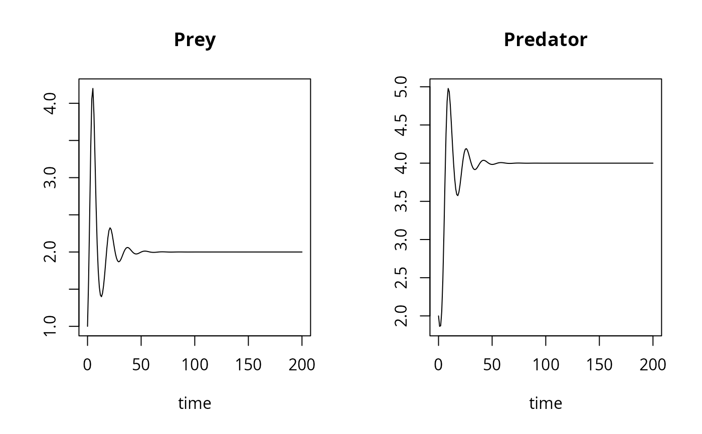
## Example1: Predator-Prey Lotka-Volterra model (with logistic prey)
## =======================================================================
LVmod <- function(Time, State, Pars) {
with(as.list(c(State, Pars)), {
Ingestion <- rIng * Prey * Predator
GrowthPrey <- rGrow * Prey * (1 - Prey/K)
MortPredator <- rMort * Predator
dPrey <- GrowthPrey - Ingestion
dPredator <- Ingestion * assEff - MortPredator
return(list(c(dPrey, dPredator)))
})
}
pars <- c(rIng = 0.2, # /day, rate of ingestion
rGrow = 1.0, # /day, growth rate of prey
rMort = 0.2 , # /day, mortality rate of predator
assEff = 0.5, # -, assimilation efficiency
K = 10) # mmol/m3, carrying capacity
yini <- c(Prey = 1, Predator = 2)
times <- seq(0, 200, by = 1)
out <- ode(yini, times, LVmod, pars)
summary(out)
#> Prey Predator
#> Min. 1.0000000 1.8632829
#> 1st Qu. 1.9999571 3.9999115
#> Median 2.0000000 4.0000000
#> Mean 2.0317905 3.9606228
#> 3rd Qu. 2.0000751 4.0000418
#> Max. 4.2001812 4.9787222
#> N 201.0000000 201.0000000
#> sd 0.3138139 0.3489079
## Default plot method
plot(out)
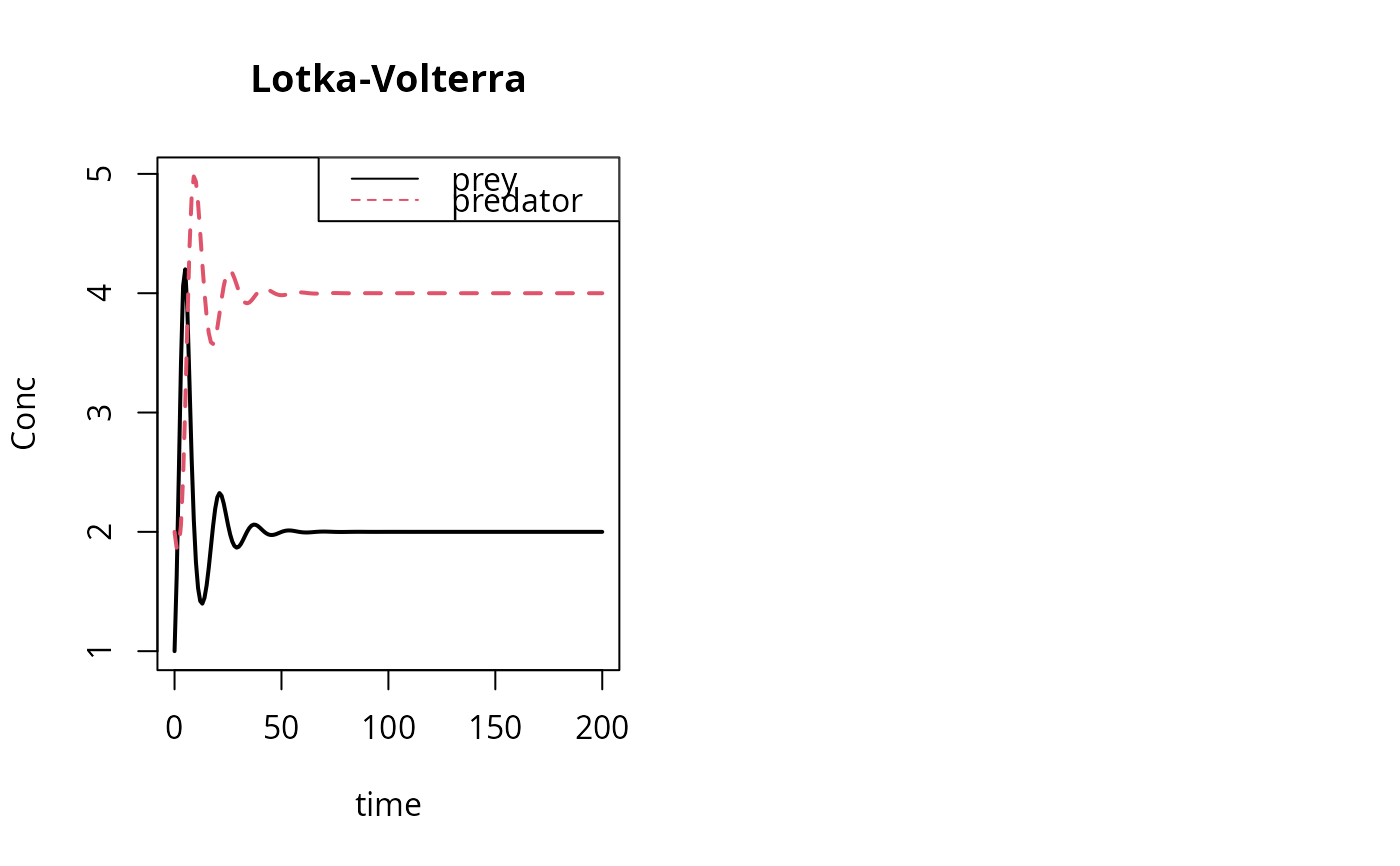
 ## User specified plotting
matplot(out[ , 1], out[ , 2:3], type = "l", xlab = "time", ylab = "Conc",
main = "Lotka-Volterra", lwd = 2)
legend("topright", c("prey", "predator"), col = 1:2, lty = 1:2)
## =======================================================================
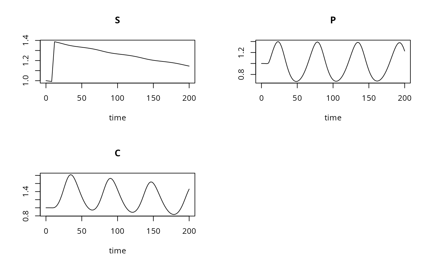
## Example2: Substrate-Producer-Consumer Lotka-Volterra model
## =======================================================================
## Note:
## Function sigimp passed as an argument (input) to model
## (see also lsoda and rk examples)
SPCmod <- function(t, x, parms, input) {
with(as.list(c(parms, x)), {
import <- input(t)
dS <- import - b*S*P + g*C # substrate
dP <- c*S*P - d*C*P # producer
dC <- e*P*C - f*C # consumer
res <- c(dS, dP, dC)
list(res)
})
}
## The parameters
parms <- c(b = 0.001, c = 0.1, d = 0.1, e = 0.1, f = 0.1, g = 0.0)
## vector of timesteps
times <- seq(0, 200, length = 101)
## external signal with rectangle impulse
signal <- data.frame(times = times,
import = rep(0, length(times)))
signal$import[signal$times >= 10 & signal$times <= 11] <- 0.2
sigimp <- approxfun(signal$times, signal$import, rule = 2)
## Start values for steady state
xstart <- c(S = 1, P = 1, C = 1)
## Solve model
out <- ode(y = xstart, times = times,
func = SPCmod, parms = parms, input = sigimp)
## Default plot method
plot(out)
## User specified plotting
matplot(out[ , 1], out[ , 2:3], type = "l", xlab = "time", ylab = "Conc",
main = "Lotka-Volterra", lwd = 2)
legend("topright", c("prey", "predator"), col = 1:2, lty = 1:2)
## =======================================================================
## Example2: Substrate-Producer-Consumer Lotka-Volterra model
## =======================================================================
## Note:
## Function sigimp passed as an argument (input) to model
## (see also lsoda and rk examples)
SPCmod <- function(t, x, parms, input) {
with(as.list(c(parms, x)), {
import <- input(t)
dS <- import - b*S*P + g*C # substrate
dP <- c*S*P - d*C*P # producer
dC <- e*P*C - f*C # consumer
res <- c(dS, dP, dC)
list(res)
})
}
## The parameters
parms <- c(b = 0.001, c = 0.1, d = 0.1, e = 0.1, f = 0.1, g = 0.0)
## vector of timesteps
times <- seq(0, 200, length = 101)
## external signal with rectangle impulse
signal <- data.frame(times = times,
import = rep(0, length(times)))
signal$import[signal$times >= 10 & signal$times <= 11] <- 0.2
sigimp <- approxfun(signal$times, signal$import, rule = 2)
## Start values for steady state
xstart <- c(S = 1, P = 1, C = 1)
## Solve model
out <- ode(y = xstart, times = times,
func = SPCmod, parms = parms, input = sigimp)
## Default plot method
plot(out)
 ## User specified plotting
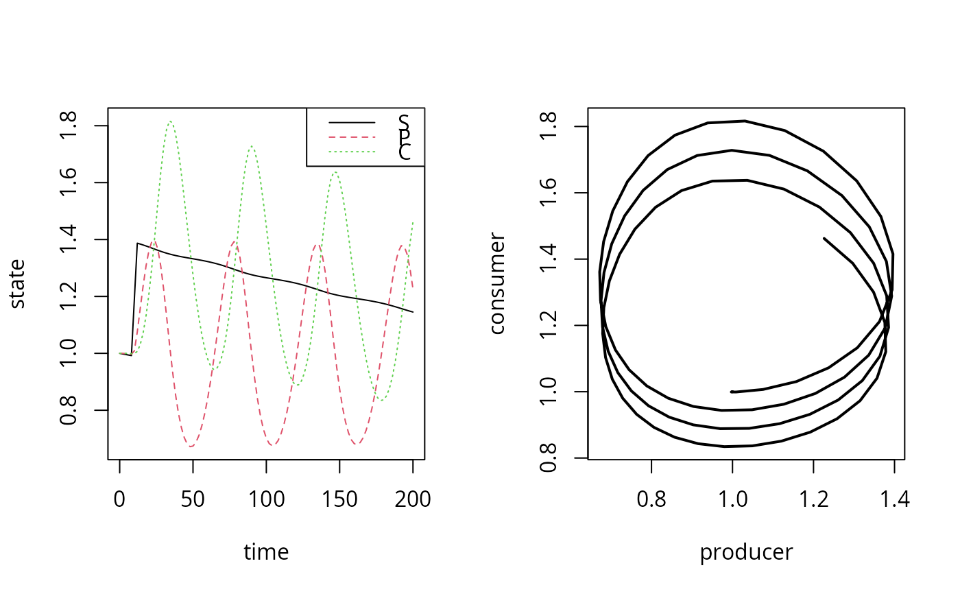
mf <- par(mfrow = c(1, 2))
## User specified plotting
mf <- par(mfrow = c(1, 2))
 matplot(out[,1], out[,2:4], type = "l", xlab = "time", ylab = "state")
legend("topright", col = 1:3, lty = 1:3, legend = c("S", "P", "C"))
plot(out[,"P"], out[,"C"], type = "l", lwd = 2, xlab = "producer",
ylab = "consumer")
matplot(out[,1], out[,2:4], type = "l", xlab = "time", ylab = "state")
legend("topright", col = 1:3, lty = 1:3, legend = c("S", "P", "C"))
plot(out[,"P"], out[,"C"], type = "l", lwd = 2, xlab = "producer",
ylab = "consumer")
 par(mfrow = mf)
## =======================================================================
## Example3: Discrete time model - using method = "iteration"
## The host-parasitoid model from Soetaert and Herman, 2009,
## Springer - p. 284.
## =======================================================================
Parasite <- function(t, y, ks) {
P <- y[1]
H <- y[2]
f <- A * P / (ks + H)
Pnew <- H * (1 - exp(-f))
Hnew <- H * exp(rH * (1 - H) - f)
list (c(Pnew, Hnew))
}
rH <- 2.82 # rate of increase
A <- 100 # attack rate
ks <- 15 # half-saturation density
out <- ode(func = Parasite, y = c(P = 0.5, H = 0.5), times = 0:50, parms = ks,
method = "iteration")
out2<- ode(func = Parasite, y = c(P = 0.5, H = 0.5), times = 0:50, parms = 25,
method = "iteration")
out3<- ode(func = Parasite, y = c(P = 0.5, H = 0.5), times = 0:50, parms = 35,
method = "iteration")
## Plot all 3 scenarios in one figure
plot(out, out2, out3, lty = 1, lwd = 2)
par(mfrow = mf)
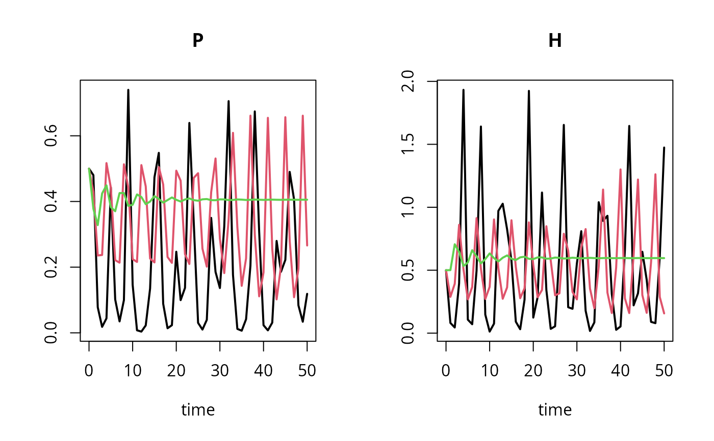
## =======================================================================
## Example3: Discrete time model - using method = "iteration"
## The host-parasitoid model from Soetaert and Herman, 2009,
## Springer - p. 284.
## =======================================================================
Parasite <- function(t, y, ks) {
P <- y[1]
H <- y[2]
f <- A * P / (ks + H)
Pnew <- H * (1 - exp(-f))
Hnew <- H * exp(rH * (1 - H) - f)
list (c(Pnew, Hnew))
}
rH <- 2.82 # rate of increase
A <- 100 # attack rate
ks <- 15 # half-saturation density
out <- ode(func = Parasite, y = c(P = 0.5, H = 0.5), times = 0:50, parms = ks,
method = "iteration")
out2<- ode(func = Parasite, y = c(P = 0.5, H = 0.5), times = 0:50, parms = 25,
method = "iteration")
out3<- ode(func = Parasite, y = c(P = 0.5, H = 0.5), times = 0:50, parms = 35,
method = "iteration")
## Plot all 3 scenarios in one figure
plot(out, out2, out3, lty = 1, lwd = 2)
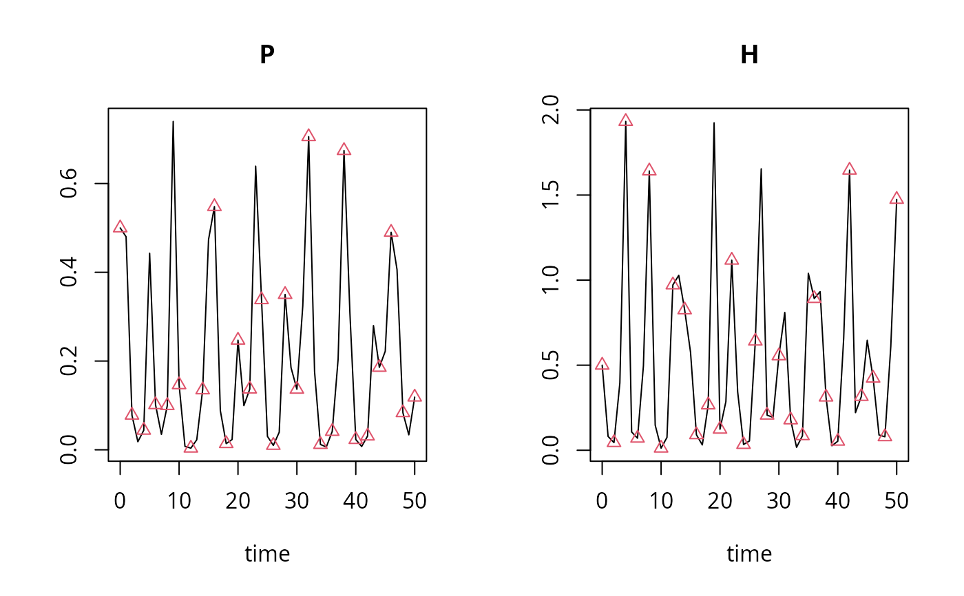
 ## Same like "out", but *output* every two steps
## hini = 1 ensures that the same *internal* timestep of 1 is used
outb <- ode(func = Parasite, y = c(P = 0.5, H = 0.5),
times = seq(0, 50, 2), hini = 1, parms = ks,
method = "iteration")
plot(out, outb, type = c("l", "p"))
## Same like "out", but *output* every two steps
## hini = 1 ensures that the same *internal* timestep of 1 is used
outb <- ode(func = Parasite, y = c(P = 0.5, H = 0.5),
times = seq(0, 50, 2), hini = 1, parms = ks,
method = "iteration")
plot(out, outb, type = c("l", "p"))
 if (FALSE) { # \dontrun{
## =======================================================================
## Example4: Playing with the Jacobian options - see e.g. lsoda help page
##
## IMPORTANT: The following example is temporarily broken because of
## incompatibility with R 3.0 on some systems.
## A fix is on the way.
## =======================================================================
## a stiff equation, exponential decay, run 500 times
stiff <- function(t, y, p) { # y and r are a 500-valued vector
list(- r * y)
}
N <- 500
r <- runif(N, 15, 20)
yini <- runif(N, 1, 40)
times <- 0:10
## Using the default
print(system.time(
out <- ode(y = yini, parms = NULL, times = times, func = stiff)
))
# diagnostics(out) shows that the method used = bdf (2), so it it stiff
## Specify that the Jacobian is banded, with nonzero values on the
## diagonal, i.e. the bandwidth up and down = 0
print(system.time(
out2 <- ode(y = yini, parms = NULL, times = times, func = stiff,
jactype = "bandint", bandup = 0, banddown = 0)
))
## Now we also specify the Jacobian function
jacob <- function(t, y, p) -r
print(system.time(
out3 <- ode(y = yini, parms = NULL, times = times, func = stiff,
jacfunc = jacob, jactype = "bandusr",
bandup = 0, banddown = 0)
))
## The larger the value of N, the larger the time gain...
} # }
if (FALSE) { # \dontrun{
## =======================================================================
## Example4: Playing with the Jacobian options - see e.g. lsoda help page
##
## IMPORTANT: The following example is temporarily broken because of
## incompatibility with R 3.0 on some systems.
## A fix is on the way.
## =======================================================================
## a stiff equation, exponential decay, run 500 times
stiff <- function(t, y, p) { # y and r are a 500-valued vector
list(- r * y)
}
N <- 500
r <- runif(N, 15, 20)
yini <- runif(N, 1, 40)
times <- 0:10
## Using the default
print(system.time(
out <- ode(y = yini, parms = NULL, times = times, func = stiff)
))
# diagnostics(out) shows that the method used = bdf (2), so it it stiff
## Specify that the Jacobian is banded, with nonzero values on the
## diagonal, i.e. the bandwidth up and down = 0
print(system.time(
out2 <- ode(y = yini, parms = NULL, times = times, func = stiff,
jactype = "bandint", bandup = 0, banddown = 0)
))
## Now we also specify the Jacobian function
jacob <- function(t, y, p) -r
print(system.time(
out3 <- ode(y = yini, parms = NULL, times = times, func = stiff,
jacfunc = jacob, jactype = "bandusr",
bandup = 0, banddown = 0)
))
## The larger the value of N, the larger the time gain...
} # }