General Solver for Delay Differential Equations.

Function dede is a general solver for delay differential equations, i.e. equations where the derivative depends on past values of the state variables or their derivatives.

Usage

dede(y, times, func=NULL, parms,
    method = c( "lsoda", "lsode", "lsodes", "lsodar", "vode",
       "daspk", "bdf", "adams", "impAdams", "radau"), control = NULL, ...)

Arguments

y

the initial (state) values for the DE system, a vector. If y has a name attribute, the names will be used to label the output matrix.

times

time sequence for which output is wanted; the first value of times must be the initial time.

func

an R-function that computes the values of the derivatives in the ODE system (the model definition) at time $t$.

func must be defined as: func <- function(t, y, parms, ...). t is the current time point in the integration, y is the current estimate of the variables in the DE system. If the initial values y has a names attribute, the names will be available inside func. parms is a vector or list of parameters; ... (optional) are any other arguments passed to the function.

The return value of func should be a list, whose first element is a vector containing the derivatives of y with respect to time, and whose next elements are global values that are required at each point in times.The derivatives must be specified in the same order as the state variables y.

If method "daspk" is used, then func can be NULL, in which case res should be used.

parms

parameters passed to func.

method

the integrator to use, either a string ("lsoda", "lsode", "lsodes", "lsodar", "vode", "daspk", "bdf", "adams", "impAdams", "radau") or a function that performs the integration. The default integrator used is lsoda.

control

a list that can supply (1) the size of the history array, as control$mxhist; the default is 1e4 and (2) how to interpolate, as control$interpol, where 1 is hermitian interpolation, 2 is variable order interpolation, using the Nordsieck history array. Only for the two Adams methods is the second option recommended.

...

additional arguments passed to the integrator.

Value

A matrix of class deSolve with up to as many rows as elements in times and as many columns as elements in y plus the number of "global" values returned in the second element of the return from func, plus an additional column (the first) for the time value. There will be one row for each element in times unless the integrator returns with an unrecoverable error. If y has a names attribute, it will be used to label the columns of the output value.

Author

Karline Soetaert <karline.soetaert@nioz.nl>

Details

Functions lagvalue and lagderiv are to be used with dede as they provide access to past (lagged) values of state variables and derivatives. The number of past values that are to be stored in a history matrix, can be specified in control$mxhist. The default value (if unspecified) is 1e4.

Cubic Hermite interpolation is used by default to obtain an accurate interpolant at the requested lagged time. For methods adams, impAdams, a more accurate interpolation method can be triggered by setting control$interpol = 2.

dede does not deal explicitly with propagated derivative discontinuities, but relies on the integrator to control the stepsize in the region of a discontinuity.

dede does not include methods to deal with delays that are smaller than the stepsize, although in some cases it may be possible to solve such models.

For these reasons, it can only solve rather simple delay differential equations.

When used together with integrator lsodar, or lsode, dde can simultaneously locate a root, and trigger an event. See last example.

Examples

## =============================================================================
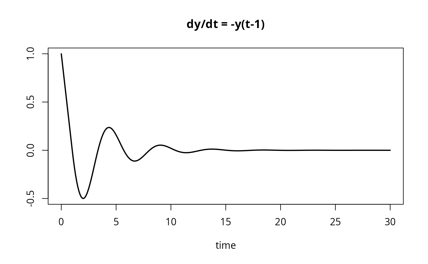
## A simple delay differential equation
## dy(t) = -y(t-1) ; y(t<0)=1
## =============================================================================

##-----------------------------
## the derivative function
##-----------------------------
derivs <- function(t, y, parms) {
  if (t < 1)
    dy <- -1
  else
    dy <- - lagvalue(t - 1)
  list(c(dy))
}

##-----------------------------
## initial values and times
##-----------------------------
yinit <- 1
times <- seq(0, 30, 0.1)

##-----------------------------
## solve the model
##-----------------------------
yout <- dede(y = yinit, times = times, func = derivs, parms = NULL)

##-----------------------------
## display, plot results
##-----------------------------
plot(yout, type = "l", lwd = 2, main = "dy/dt = -y(t-1)")


## =============================================================================
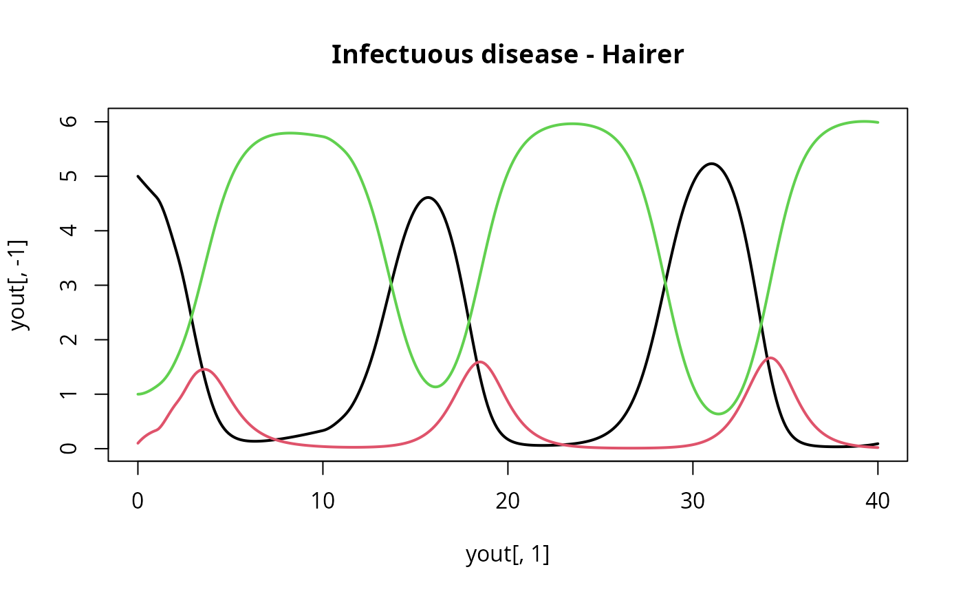
## The infectuous disease model of Hairer; two lags.
## example 4 from Shampine and Thompson, 2000
## solving delay differential equations with dde23
## =============================================================================

##-----------------------------
## the derivative function
##-----------------------------
derivs <- function(t,y,parms) {
  if (t < 1)
    lag1 <- 0.1
  else
    lag1 <- lagvalue(t - 1,2)
  if (t < 10)
    lag10 <- 0.1
  else
    lag10 <- lagvalue(t - 10,2)

  dy1 <- -y[1] * lag1 + lag10
  dy2 <-  y[1] * lag1 - y[2]
  dy3 <-  y[2] - lag10
  list(c(dy1, dy2, dy3))
}

##-----------------------------
## initial values and times
##-----------------------------
yinit <- c(5, 0.1, 1)
times <- seq(0, 40, by = 0.1)

##-----------------------------
## solve the model
##-----------------------------
system.time(
  yout <- dede(y = yinit, times = times, func = derivs, parms = NULL)
)
#>    user  system elapsed 
#>   0.037   0.000   0.036 

##-----------------------------
## display, plot results
##-----------------------------
matplot(yout[,1], yout[,-1], type = "l", lwd = 2, lty = 1,
  main = "Infectuous disease - Hairer")


## =============================================================================
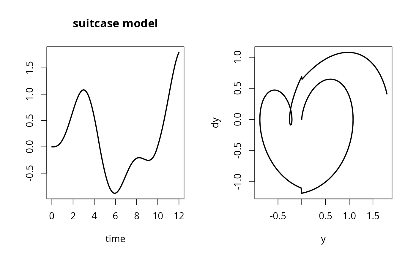
## time lags + EVENTS triggered by a root function
## The two-wheeled suitcase model
## example 8 from Shampine and Thompson, 2000
## solving delay differential equations with dde23
## =============================================================================

##-----------------------------
## the derivative function
##-----------------------------
derivs <- function(t, y, parms) {
  if (t < tau)
    lag <- 0
  else
    lag <- lagvalue(t - tau)

  dy1 <- y[2]
  dy2 <- -sign(y[1]) * gam * cos(y[1]) +
          sin(y[1]) - bet * lag[1] + A * sin(omega * t + mu)
  list(c(dy1, dy2))
}

## root and event function
root <- function(t,y,parms) ifelse(t>0, return(y), return(1))
event <- function(t,y,parms) return(c(y[1], y[2]*0.931))

gam = 0.248; bet = 1; tau = 0.1; A = 0.75
omega = 1.37; mu = asin(gam/A)

##-----------------------------
## initial values and times
##-----------------------------
yinit <- c(y = 0, dy = 0)
times <- seq(0, 12, len = 1000)

##-----------------------------
## solve the model
##-----------------------------
## Note: use a solver that supports both root finding and events,
##       e.g. lsodar, lsode, lsoda, adams, bdf
yout <- dede(y = yinit, times = times, func = derivs, parms = NULL,
  method = "lsodar", rootfun = root, events = list(func = event, root = TRUE))

##-----------------------------
## display, plot results
##-----------------------------

plot(yout, which = 1, type = "l", lwd = 2, main = "suitcase model", mfrow = c(1,2))
plot(yout[,2], yout[,3], xlab = "y", ylab = "dy", type = "l", lwd = 2)