Solver for Ordinary Differential Equations (ODE)

Solves the initial value problem for stiff or nonstiff systems of ordinary differential equations (ODE) in the form: $$dy/dt = f(t,y)$$.

The R function lsode provides an interface to the FORTRAN ODE solver of the same name, written by Alan C. Hindmarsh and Andrew H. Sherman.

It combines parts of the code lsodar and can thus find the root of at least one of a set of constraint functions g(i) of the independent and dependent variables. This can be used to stop the simulation or to trigger events, i.e. a sudden change in one of the state variables.

The system of ODE's is written as an R function or be defined in compiled code that has been dynamically loaded.

In contrast to lsoda, the user has to specify whether or not the problem is stiff and choose the appropriate solution method.

lsode is very similar to vode, but uses a fixed-step-interpolate method rather than the variable-coefficient method in vode. In addition, in vode it is possible to choose whether or not a copy of the Jacobian is saved for reuse in the corrector iteration algorithm; In lsode, a copy is not kept.

Usage

lsode(y, times, func, parms, rtol = 1e-6, atol = 1e-6,  
  jacfunc = NULL, jactype = "fullint", mf = NULL, rootfunc = NULL,
  verbose = FALSE, nroot = 0, tcrit = NULL, hmin = 0, hmax = NULL, 
  hini = 0, ynames = TRUE, maxord = NULL, bandup = NULL, banddown = NULL,
  maxsteps = 5000, dllname = NULL, initfunc = dllname,
  initpar = parms, rpar = NULL, ipar = NULL, nout = 0,
  outnames = NULL, forcings=NULL, initforc = NULL, 
  fcontrol=NULL, events=NULL, lags = NULL,...)

Arguments

y

the initial (state) values for the ODE system. If y has a name attribute, the names will be used to label the output matrix.

times

time sequence for which output is wanted; the first value of times must be the initial time; if only one step is to be taken; set times = NULL.

func

either an R-function that computes the values of the derivatives in the ODE system (the model definition) at time t, or a character string giving the name of a compiled function in a dynamically loaded shared library.

If func is an R-function, it must be defined as: func <- function(t, y, parms,...). t is the current time point in the integration, y is the current estimate of the variables in the ODE system. If the initial values y has a names attribute, the names will be available inside func. parms is a vector or list of parameters; ... (optional) are any other arguments passed to the function.

The return value of func should be a list, whose first element is a vector containing the derivatives of y with respect to time, and whose next elements are global values that are required at each point in times. The derivatives must be specified in the same order as the state variables y.

If func is a string, then dllname must give the name of the shared library (without extension) which must be loaded before lsode() is called. See package vignette "compiledCode" for more details.

parms

vector or list of parameters used in func or jacfunc.

rtol

relative error tolerance, either a scalar or an array as long as y. See details.

atol

absolute error tolerance, either a scalar or an array as long as y. See details.

jacfunc

if not NULL, an R function that computes the Jacobian of the system of differential equations $\partial\dot{y}_i/\partial y_j$, or a string giving the name of a function or subroutine in dllname that computes the Jacobian (see vignette "compiledCode" for more about this option).

In some circumstances, supplying jacfunc can speed up the computations, if the system is stiff. The R calling sequence for jacfunc is identical to that of func.

If the Jacobian is a full matrix, jacfunc should return a matrix $\partial\dot{y}/\partial y$, where the ith row contains the derivative of $dy_i/dt$ with respect to $y_j$, or a vector containing the matrix elements by columns (the way R and FORTRAN store matrices).
If the Jacobian is banded, jacfunc should return a matrix containing only the nonzero bands of the Jacobian, rotated row-wise. See first example of lsode.

jactype

the structure of the Jacobian, one of "fullint", "fullusr", "bandusr" or "bandint" - either full or banded and estimated internally or by user; overruled if mfis not NULL.

mf

the "method flag" passed to function lsode - overrules jactype - provides more options than jactype - see details.

rootfunc

if not NULL, an R function that computes the function whose root has to be estimated or a string giving the name of a function or subroutine in dllname that computes the root function. The R calling sequence for rootfunc is identical to that of func. rootfunc should return a vector with the function values whose root is sought.

verbose

if TRUE: full output to the screen, e.g. will print the diagnostiscs of the integration - see details.

nroot

only used if dllname is specified: the number of constraint functions whose roots are desired during the integration; if rootfunc is an R-function, the solver estimates the number of roots.

tcrit

if not NULL, then lsode cannot integrate past tcrit. The FORTRAN routine lsode overshoots its targets (times points in the vector times), and interpolates values for the desired time points. If there is a time beyond which integration should not proceed (perhaps because of a singularity), that should be provided in tcrit.

hmin

an optional minimum value of the integration stepsize. In special situations this parameter may speed up computations with the cost of precision. Don't use hmin if you don't know why!

hmax

an optional maximum value of the integration stepsize. If not specified, hmax is set to the largest difference in times, to avoid that the simulation possibly ignores short-term events. If 0, no maximal size is specified.

hini

initial step size to be attempted; if 0, the initial step size is determined by the solver.

ynames

logical, if FALSE names of state variables are not passed to function func; this may speed up the simulation especially for multi-D models.

maxord

the maximum order to be allowed. NULL uses the default, i.e. order 12 if implicit Adams method (meth = 1), order 5 if BDF method (meth = 2). Reduce maxord to save storage space.

bandup

number of non-zero bands above the diagonal, in case the Jacobian is banded.

banddown

number of non-zero bands below the diagonal, in case the Jacobian is banded.

maxsteps

maximal number of steps per output interval taken by the solver.

dllname

a string giving the name of the shared library (without extension) that contains all the compiled function or subroutine definitions refered to in func and jacfunc. See package vignette "compiledCode".

initfunc

if not NULL, the name of the initialisation function (which initialises values of parameters), as provided in dllname. See package vignette "compiledCode".

initpar

only when dllname is specified and an initialisation function initfunc is in the dll: the parameters passed to the initialiser, to initialise the common blocks (FORTRAN) or global variables (C, C++).

rpar

only when dllname is specified: a vector with double precision values passed to the dll-functions whose names are specified by func and jacfunc.

ipar

only when dllname is specified: a vector with integer values passed to the dll-functions whose names are specified by func and jacfunc.

nout

only used if dllname is specified and the model is defined in compiled code: the number of output variables calculated in the compiled function func, present in the shared library. Note: it is not automatically checked whether this is indeed the number of output variables calculated in the dll - you have to perform this check in the code - See package vignette "compiledCode".

outnames

only used if dllname is specified and nout > 0: the names of output variables calculated in the compiled function func, present in the shared library. These names will be used to label the output matrix.

forcings

only used if dllname is specified: a list with the forcing function data sets, each present as a two-columned matrix, with (time,value); interpolation outside the interval [min(times), max(times)] is done by taking the value at the closest data extreme.

See forcings or package vignette "compiledCode".

initforc

if not NULL, the name of the forcing function initialisation function, as provided in dllname. It MUST be present if forcings has been given a value. See forcings or package vignette "compiledCode".

fcontrol

A list of control parameters for the forcing functions. See forcings or vignette compiledCode.

events

A matrix or data frame that specifies events, i.e. when the value of a state variable is suddenly changed. See events for more information.

lags

A list that specifies timelags, i.e. the number of steps that has to be kept. To be used for delay differential equations. See timelags, dede for more information.

...

additional arguments passed to func and jacfunc allowing this to be a generic function.

Value

A matrix of class deSolve with up to as many rows as elements in times and as many columns as elements in y plus the number of "global" values returned in the next elements of the return from func, plus and additional column for the time value. There will be a row for each element in times unless the FORTRAN routine `lsode' returns with an unrecoverable error. If y has a names attribute, it will be used to label the columns of the output value.

Author

Karline Soetaert <karline.soetaert@nioz.nl>

References

Alan C. Hindmarsh, "ODEPACK, A Systematized Collection of ODE Solvers," in Scientific Computing, R. S. Stepleman, et al., Eds. (North-Holland, Amsterdam, 1983), pp. 55-64.

Details

The work is done by the FORTRAN subroutine lsode, whose documentation should be consulted for details (it is included as comments in the source file src/opkdmain.f). The implementation is based on the November, 2003 version of lsode, from Netlib.

Before using the integrator lsode, the user has to decide whether or not the problem is stiff.

If the problem is nonstiff, use method flag mf = 10, which selects a nonstiff (Adams) method, no Jacobian used.
If the problem is stiff, there are four standard choices which can be specified with jactype or mf.

The options for jactype are

jactype = "fullint": a full Jacobian, calculated internally by lsode, corresponds to mf = 22,
jactype = "fullusr": a full Jacobian, specified by user function jacfunc, corresponds to mf = 21,
jactype = "bandusr": a banded Jacobian, specified by user function jacfunc; the size of the bands specified by bandup and banddown, corresponds to mf = 24,
jactype = "bandint": a banded Jacobian, calculated by lsode; the size of the bands specified by bandup and banddown, corresponds to mf = 25.

More options are available when specifying mf directly.
The legal values of mf are 10, 11, 12, 13, 14, 15, 20, 21, 22, 23, 24, 25.
mf is a positive two-digit integer, mf = (10*METH + MITER), where

METH: indicates the basic linear multistep method: METH = 1 means the implicit Adams method. METH = 2 means the method based on backward differentiation formulas (BDF-s).
MITER: indicates the corrector iteration method: MITER = 0 means functional iteration (no Jacobian matrix is involved). MITER = 1 means chord iteration with a user-supplied full (NEQ by NEQ) Jacobian. MITER = 2 means chord iteration with an internally generated (difference quotient) full Jacobian (using NEQ extra calls to func per df/dy value). MITER = 3 means chord iteration with an internally generated diagonal Jacobian approximation (using 1 extra call to func per df/dy evaluation). MITER = 4 means chord iteration with a user-supplied banded Jacobian. MITER = 5 means chord iteration with an internally generated banded Jacobian (using ML+MU+1 extra calls to func per df/dy evaluation).

If MITER = 1 or 4, the user must supply a subroutine jacfunc.

Inspection of the example below shows how to specify both a banded and full Jacobian.

The input parameters rtol, and atol determine the error control performed by the solver. See lsoda for details.

The diagnostics of the integration can be printed to screen by calling diagnostics. If verbose = TRUE, the diagnostics will written to the screen at the end of the integration.

See vignette("deSolve") for an explanation of each element in the vectors containing the diagnostic properties and how to directly access them.

Models may be defined in compiled C or FORTRAN code, as well as in an R-function. See package vignette "compiledCode" for details.

More information about models defined in compiled code is in the package vignette ("compiledCode"); information about linking forcing functions to compiled code is in forcings.

Examples in both C and FORTRAN are in the dynload subdirectory of the deSolve package directory.

lsode can find the root of at least one of a set of constraint functions rootfunc of the independent and dependent variables. It then returns the solution at the root if that occurs sooner than the specified stop condition, and otherwise returns the solution according the specified stop condition.

Caution: Because of numerical errors in the function rootfun due to roundoff and integration error, lsode may return false roots, or return the same root at two or more nearly equal values of time.

Examples

## =======================================================================
## Example 1:
##   Various ways to solve the same model.
## =======================================================================

## the model, 5 state variables
f1 <- function  (t, y, parms) {
  ydot <- vector(len = 5)

  ydot[1] <-  0.1*y[1] -0.2*y[2]
  ydot[2] <- -0.3*y[1] +0.1*y[2] -0.2*y[3]
  ydot[3] <-           -0.3*y[2] +0.1*y[3] -0.2*y[4]
  ydot[4] <-                     -0.3*y[3] +0.1*y[4] -0.2*y[5]
  ydot[5] <-                               -0.3*y[4] +0.1*y[5]

  return(list(ydot))
}

## the Jacobian, written as a full matrix
fulljac <- function  (t, y, parms) {
  jac <- matrix(nrow = 5, ncol = 5, byrow = TRUE,
                data = c(0.1, -0.2,  0  ,  0  ,  0  ,
                        -0.3,  0.1, -0.2,  0  ,  0  ,
                         0  , -0.3,  0.1, -0.2,  0  ,
                         0  ,  0  , -0.3,  0.1, -0.2,
                         0  ,  0  ,  0  , -0.3,  0.1))
  return(jac)
}

## the Jacobian, written in banded form
bandjac <- function  (t, y, parms) {
  jac <- matrix(nrow = 3, ncol = 5, byrow = TRUE,
                data = c( 0  , -0.2, -0.2, -0.2, -0.2,
                          0.1,  0.1,  0.1,  0.1,  0.1,
                         -0.3, -0.3, -0.3, -0.3,    0))
  return(jac)
}

## initial conditions and output times
yini  <- 1:5
times <- 1:20

## default: stiff method, internally generated, full Jacobian
out   <- lsode(yini, times, f1, parms = 0, jactype = "fullint")

## stiff method, user-generated full Jacobian
out2  <- lsode(yini, times, f1, parms = 0, jactype = "fullusr",
              jacfunc = fulljac)

## stiff method, internally-generated banded Jacobian
## one nonzero band above (up) and below(down) the diagonal
out3  <- lsode(yini, times, f1, parms = 0, jactype = "bandint",
                              bandup = 1, banddown = 1)

## stiff method, user-generated banded Jacobian
out4  <- lsode(yini, times, f1, parms = 0, jactype = "bandusr",
              jacfunc = bandjac, bandup = 1, banddown = 1)

## non-stiff method
out5  <- lsode(yini, times, f1, parms = 0, mf = 10)

## =======================================================================
## Example 2:
##   diffusion on a 2-D grid
##   partially specified Jacobian
## =======================================================================

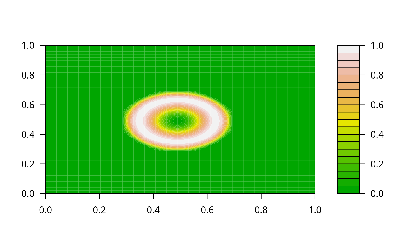
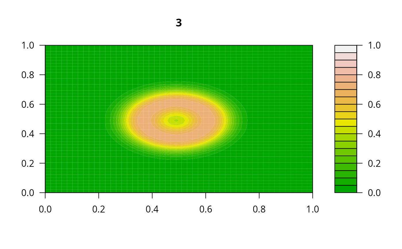
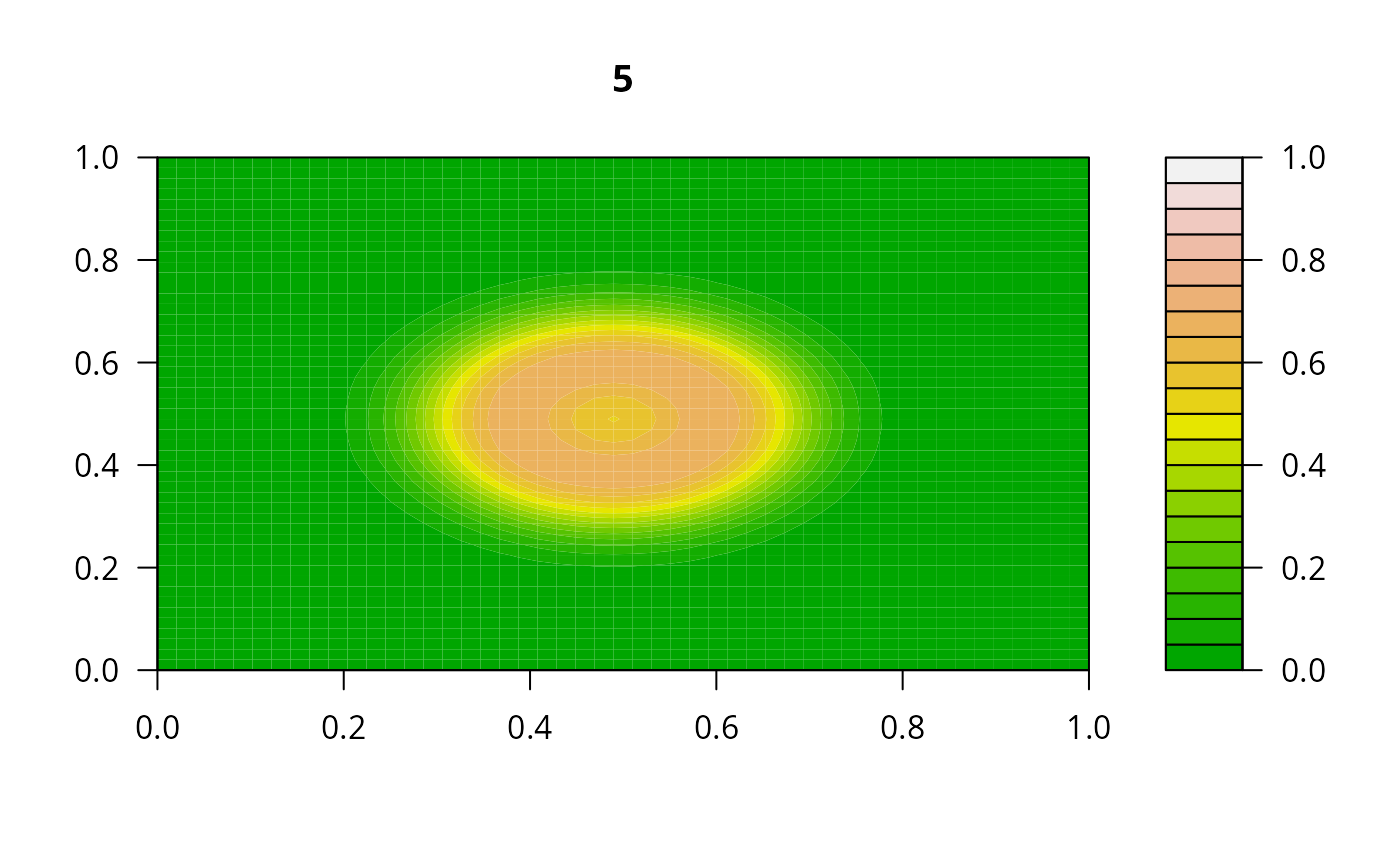
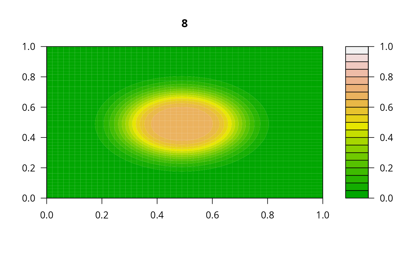
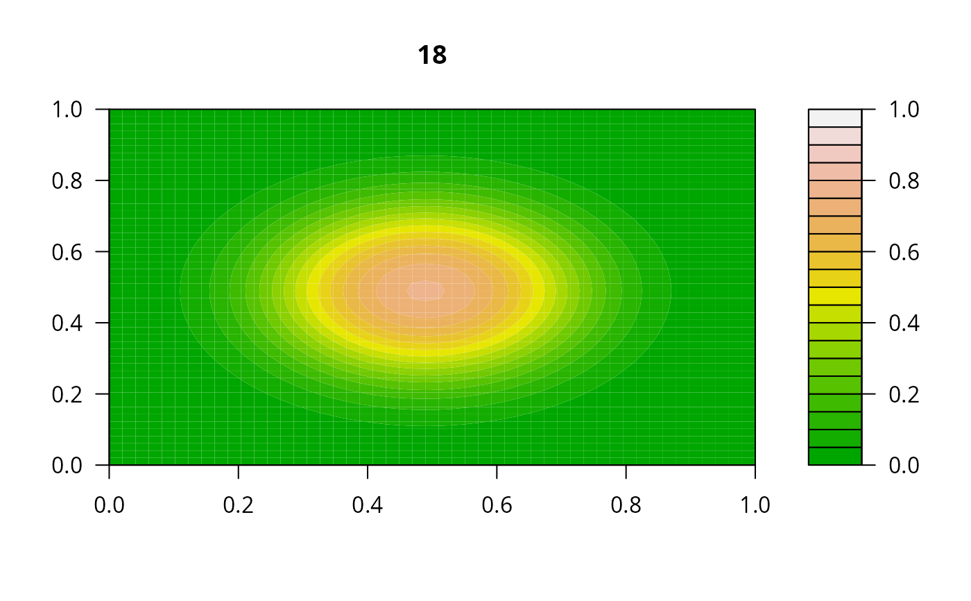
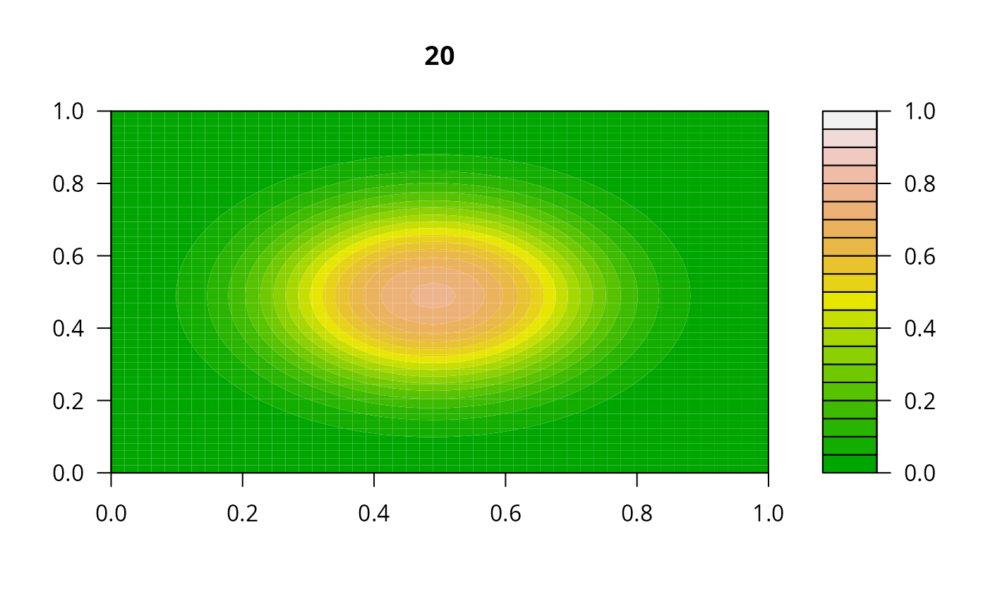
diffusion2D <- function(t, Y, par) {
   y <- matrix(nrow = n, ncol = n, data = Y)
   dY   <- r*y     # production

   ## diffusion in X-direction; boundaries = 0-concentration
   Flux <- -Dx * rbind(y[1,],(y[2:n,]-y[1:(n-1),]),-y[n,])/dx
   dY   <- dY - (Flux[2:(n+1),]-Flux[1:n,])/dx

   ## diffusion in Y-direction
   Flux <- -Dy * cbind(y[,1],(y[,2:n]-y[,1:(n-1)]),-y[,n])/dy
   dY    <- dY - (Flux[,2:(n+1)]-Flux[,1:n])/dy

   return(list(as.vector(dY)))
}

## parameters
dy    <- dx <- 1   # grid size
Dy    <- Dx <- 1   # diffusion coeff, X- and Y-direction
r     <- 0.025     # production rate
times <- c(0, 1)

n  <- 50
y  <- matrix(nrow = n, ncol = n, 0)

pa <- par(ask = FALSE)

## initial condition
for (i in 1:n) {
  for (j in 1:n) {
    dst <- (i - n/2)^2 + (j - n/2)^2
    y[i, j] <- max(0, 1 - 1/(n*n) * (dst - n)^2)
  }
}
filled.contour(y, color.palette = terrain.colors)


## =======================================================================
##   jacfunc need not be estimated exactly
##   a crude approximation, with a smaller bandwidth will do.
##   Here the half-bandwidth 1 is used, whereas the true
##   half-bandwidths are equal to n.
##   This corresponds to ignoring the y-direction coupling in the ODEs.
## =======================================================================

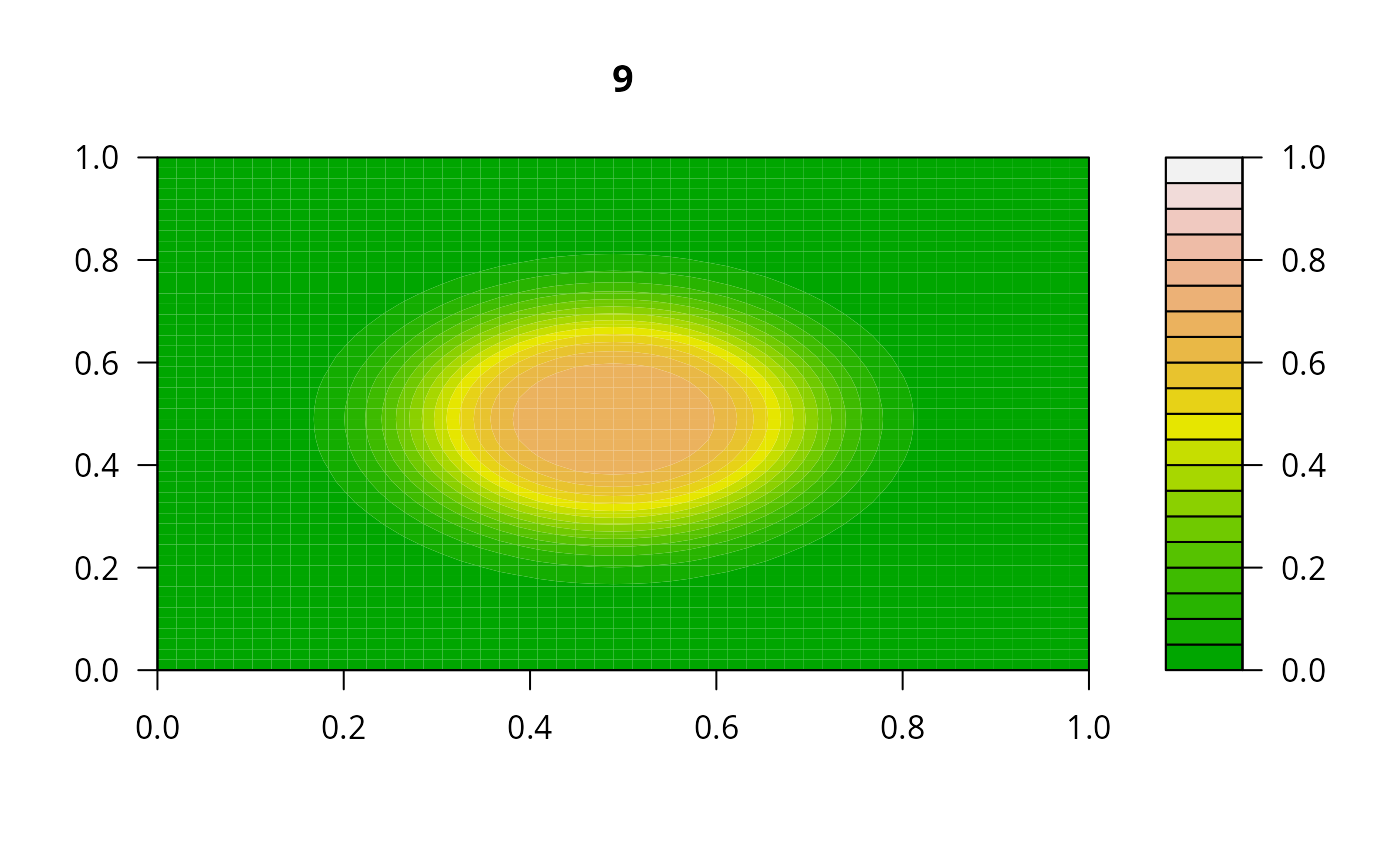
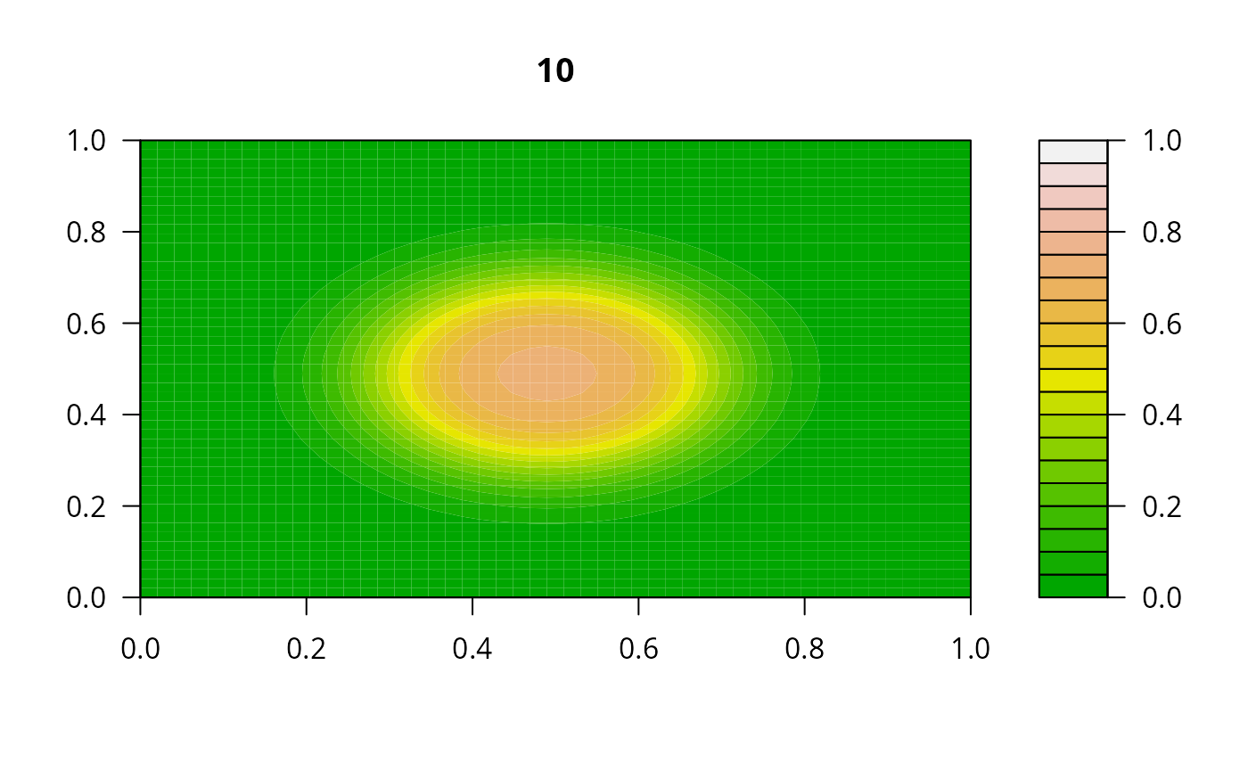
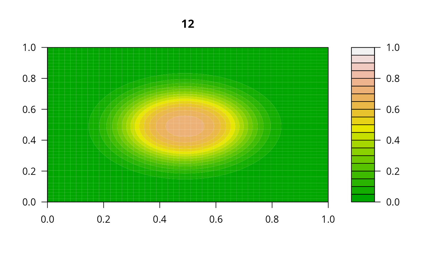
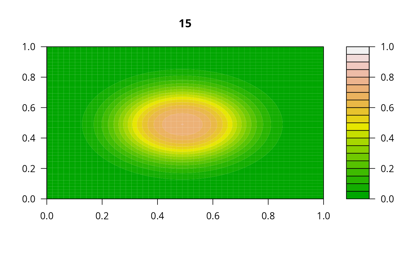
print(system.time(
  for (i in 1:20) {
    out  <-  lsode(func = diffusion2D, y = as.vector(y), times = times,
              parms = NULL, jactype = "bandint", bandup = 1, banddown = 1)

    filled.contour(matrix(nrow = n, ncol = n, out[2,-1]), zlim = c(0,1),
                  color.palette = terrain.colors, main = i)

    y <- out[2, -1]
  }
))




















#>    user  system elapsed 
#>   0.252   0.009   0.261 
par(ask = pa)