Solver For Multicomponent 1-D Ordinary Differential Equations
ode.1D.RdSolves a system of ordinary differential equations resulting from 1-Dimensional partial differential equations that have been converted to ODEs by numerical differencing.
Usage
ode.1D(y, times, func, parms, nspec = NULL, dimens = NULL,
   method= c("lsoda", "lsode", "lsodes", "lsodar", "vode", "daspk",
   "euler", "rk4", "ode23", "ode45", "radau", "bdf", "adams", "impAdams",
   "iteration"),
   names = NULL, bandwidth = 1, restructure = FALSE, ...)
Arguments
- y
the initial (state) values for the ODE system, a vector. If
yhas a name attribute, the names will be used to label the output matrix.- times
time sequence for which output is wanted; the first value of
timesmust be the initial time.- func
either an R-function that computes the values of the derivatives in the ODE system (the model definition) at time
t, or a character string giving the name of a compiled function in a dynamically loaded shared library.If
funcis an R-function, it must be defined as:func <- function(t, y, parms, ...).tis the current time point in the integration,yis the current estimate of the variables in the ODE system. If the initial valuesyhas anamesattribute, the names will be available insidefunc.parmsis a vector or list of parameters;...(optional) are any other arguments passed to the function.The return value of
funcshould be a list, whose first element is a vector containing the derivatives ofywith respect totime, and whose next elements are global values that are required at each point intimes. The derivatives must be specified in the same order as the state variablesy.If
funcis a character string then integratorlsodeswill be used. See details.- parms
parameters passed to
func.- nspec
the number of species (components) in the model. If
NULL, thendimensshould be specified.- dimens
the number of boxes in the model. If
NULL, thennspecshould be specified.- method
the integrator. Use
"vode", "lsode", "lsoda",
     "lsodar", "daspk"
, or"lsodes"if the model is very stiff;"impAdams"or"radau"may be best suited for mildly stiff problems;"euler", "rk4", "ode23", "ode45", "adams"are most efficient for non-stiff problems. Also allowed is to pass an integratorfunction. Use one of the other Runge-Kutta methods viarkMethod. For instance,method = rkMethod("ode45ck")will trigger the Cash-Karp method of order 4(5).Method
"iteration"is special in that here the functionfuncshould return the new value of the state variables rather than the rate of change. This can be used for individual based models, for difference equations, or in those cases where the integration is performed withinfunc)- names
the names of the components; used for plotting.
- bandwidth
the number of adjacent boxes over which transport occurs. Normally equal to 1 (box i only interacts with box i-1, and i+1). Values larger than 1 will not work with
method = "lsodes". Ignored if the method is explicit.- restructure
whether or not the Jacobian should be restructured. Only used if the
methodis an integrator function. Should beTRUEif the method is implicit,FALSEif explicit.- ...
additional arguments passed to the integrator.
Value
A matrix of class deSolve with up to as many rows as elements in times and as many
columns as elements in y plus the number of "global" values
returned in the second element of the return from func, plus an
additional column (the first) for the time value. There will be one
row for each element in times unless the integrator returns
with an unrecoverable error. If y has a names attribute, it
will be used to label the columns of the output value.
The output will have the attributes istate, and rstate,
two vectors with several useful elements. The first element of istate
returns the conditions under which the last call to the integrator
returned. Normal is istate = 2. If verbose = TRUE, the
settings of istate and rstate will be written to the screen. See the
help for the selected integrator for details.
Note
It is advisable though not mandatory to specify both
nspec and dimens. In this case, the solver can check
whether the input makes sense (i.e. if nspec * dimens ==
length(y)).
Details
This is the method of choice for multi-species 1-dimensional models, that are only subjected to transport between adjacent layers.
More specifically, this method is to be used if the state variables are arranged per species:
A[1], A[2], A[3],.... B[1], B[2], B[3],.... (for species A, B))
Two methods are implemented.
The default method rearranges the state variables as A[1], B[1], ... A[2], B[2], ... A[3], B[3], .... This reformulation leads to a banded Jacobian with (upper and lower) half bandwidth = number of species.
Then the selected integrator solves the banded problem.
The second method uses
lsodes. Based on the dimension of the problem, the method first calculates the sparsity pattern of the Jacobian, under the assumption that transport is only occurring between adjacent layers. Thenlsodesis called to solve the problem.As
lsodesis used to integrate, it may be necessary to specify the length of the real work array,lrw.Although a reasonable guess of
lrwis made, it is possible that this will be too low. In this case,ode.1Dwill return with an error message telling the size of the work array actually needed. In the second try then, setlrwequal to this number.For instance, if you get the error:
DLSODES- RWORK length is insufficient to proceed.
  Length needed is .ge. LENRW (=I1), exceeds LRW (=I2)
  In above message,  I1 =     27627   I2 =     25932
set
lrwequal to 27627 or a higher value
If the model is specified in compiled code (in a DLL), then option 2,
based on lsodes is the only solution method.
For single-species 1-D models, you may also use ode.band.
See the selected integrator for the additional options.
Examples
## =======================================================================
## example 1
## a predator and its prey diffusing on a flat surface
## in concentric circles
## 1-D model with using cylindrical coordinates
## Lotka-Volterra type biology
## =======================================================================
## ================
## Model equations
## ================
lvmod <- function (time, state, parms, N, rr, ri, dr, dri) {
with (as.list(parms), {
PREY <- state[1:N]
PRED <- state[(N+1):(2*N)]
## Fluxes due to diffusion
## at internal and external boundaries: zero gradient
FluxPrey <- -Da * diff(c(PREY[1], PREY, PREY[N]))/dri
FluxPred <- -Da * diff(c(PRED[1], PRED, PRED[N]))/dri
## Biology: Lotka-Volterra model
Ingestion <- rIng * PREY * PRED
GrowthPrey <- rGrow * PREY * (1-PREY/cap)
MortPredator <- rMort * PRED
## Rate of change = Flux gradient + Biology
dPREY <- -diff(ri * FluxPrey)/rr/dr +
GrowthPrey - Ingestion
dPRED <- -diff(ri * FluxPred)/rr/dr +
Ingestion * assEff - MortPredator
return (list(c(dPREY, dPRED)))
})
}
## ==================
## Model application
## ==================
## model parameters:
R <- 20 # total radius of surface, m
N <- 100 # 100 concentric circles
dr <- R/N # thickness of each layer
r <- seq(dr/2,by = dr,len = N) # distance of center to mid-layer
ri <- seq(0,by = dr,len = N+1) # distance to layer interface
dri <- dr # dispersion distances
parms <- c(Da = 0.05, # m2/d, dispersion coefficient
rIng = 0.2, # /day, rate of ingestion
rGrow = 1.0, # /day, growth rate of prey
rMort = 0.2 , # /day, mortality rate of pred
assEff = 0.5, # -, assimilation efficiency
cap = 10) # density, carrying capacity
## Initial conditions: both present in central circle (box 1) only
state <- rep(0, 2 * N)
state[1] <- state[N + 1] <- 10
## RUNNING the model:
times <- seq(0, 200, by = 1) # output wanted at these time intervals
## the model is solved by the two implemented methods:
## 1. Default: banded reformulation
print(system.time(
out <- ode.1D(y = state, times = times, func = lvmod, parms = parms,
nspec = 2, names = c("PREY", "PRED"),
N = N, rr = r, ri = ri, dr = dr, dri = dri)
))
#> user system elapsed
#> 0.104 0.000 0.104
## 2. Using sparse method
print(system.time(
out2 <- ode.1D(y = state, times = times, func = lvmod, parms = parms,
nspec = 2, names = c("PREY","PRED"),
N = N, rr = r, ri = ri, dr = dr, dri = dri,
method = "lsodes")
))
#> user system elapsed
#> 0.03 0.00 0.03
## ================
## Plotting output
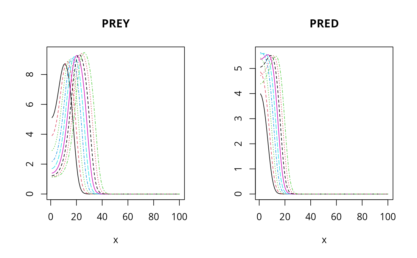
## ================
# the data in 'out' consist of: 1st col times, 2-N+1: the prey
# N+2:2*N+1: predators
PREY <- out[, 2:(N + 1)]
filled.contour(x = times, y = r, PREY, color = topo.colors,
xlab = "time, days", ylab = "Distance, m",
main = "Prey density")
 # similar:
image(out, which = "PREY", grid = r, xlab = "time, days",
legend = TRUE, ylab = "Distance, m", main = "Prey density")
# similar:
image(out, which = "PREY", grid = r, xlab = "time, days",
legend = TRUE, ylab = "Distance, m", main = "Prey density")
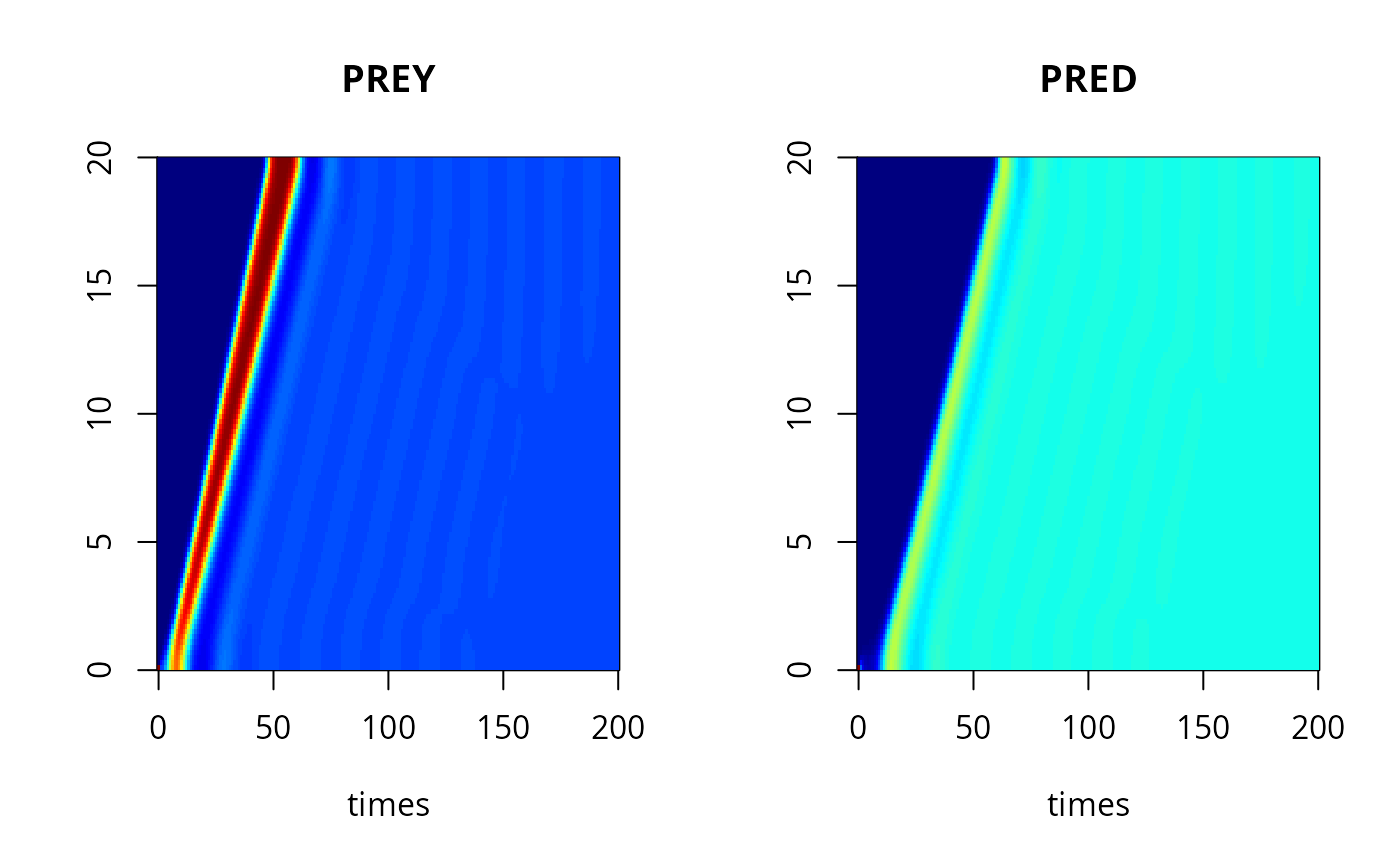
 image(out2, grid = r)
 # summaries of 1-D variables
summary(out)
#> PREY PRED
#> Min. 0.000000 0.000000
#> 1st Qu. 1.996668 3.970746
#> Median 2.000000 4.000000
#> Mean 2.094254 3.333389
#> 3rd Qu. 2.000066 4.000008
#> Max. 10.000000 10.000000
#> N 20100.000000 20100.000000
#> sd 1.648847 1.526742
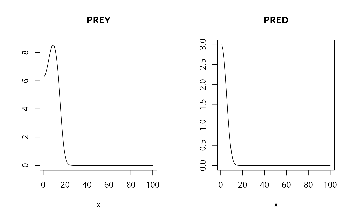
# 1-D plots:
matplot.1D(out, type = "l", subset = time == 10)
# summaries of 1-D variables
summary(out)
#> PREY PRED
#> Min. 0.000000 0.000000
#> 1st Qu. 1.996668 3.970746
#> Median 2.000000 4.000000
#> Mean 2.094254 3.333389
#> 3rd Qu. 2.000066 4.000008
#> Max. 10.000000 10.000000
#> N 20100.000000 20100.000000
#> sd 1.648847 1.526742
# 1-D plots:
matplot.1D(out, type = "l", subset = time == 10)
 matplot.1D(out, type = "l", subset = time > 10 & time < 20)
 ## =======================================================================
## Example 2.
## Biochemical Oxygen Demand (BOD) and oxygen (O2) dynamics
## in a river
## =======================================================================
## ================
## Model equations
## ================
O2BOD <- function(t, state, pars) {
BOD <- state[1:N]
O2 <- state[(N+1):(2*N)]
## BOD dynamics
FluxBOD <- v * c(BOD_0, BOD) # fluxes due to water transport
FluxO2 <- v * c(O2_0, O2)
BODrate <- r * BOD # 1-st order consumption
## rate of change = flux gradient - consumption + reaeration (O2)
dBOD <- -diff(FluxBOD)/dx - BODrate
dO2 <- -diff(FluxO2)/dx - BODrate + p * (O2sat-O2)
return(list(c(dBOD = dBOD, dO2 = dO2)))
}
## ==================
## Model application
## ==================
## parameters
dx <- 25 # grid size of 25 meters
v <- 1e3 # velocity, m/day
x <- seq(dx/2, 5000, by = dx) # m, distance from river
N <- length(x)
r <- 0.05 # /day, first-order decay of BOD
p <- 0.5 # /day, air-sea exchange rate
O2sat <- 300 # mmol/m3 saturated oxygen conc
O2_0 <- 200 # mmol/m3 riverine oxygen conc
BOD_0 <- 1000 # mmol/m3 riverine BOD concentration
## initial conditions:
state <- c(rep(200, N), rep(200, N))
times <- seq(0, 20, by = 0.1)
## running the model
## step 1 : model spinup
out <- ode.1D(y = state, times, O2BOD, parms = NULL,
nspec = 2, names = c("BOD", "O2"))
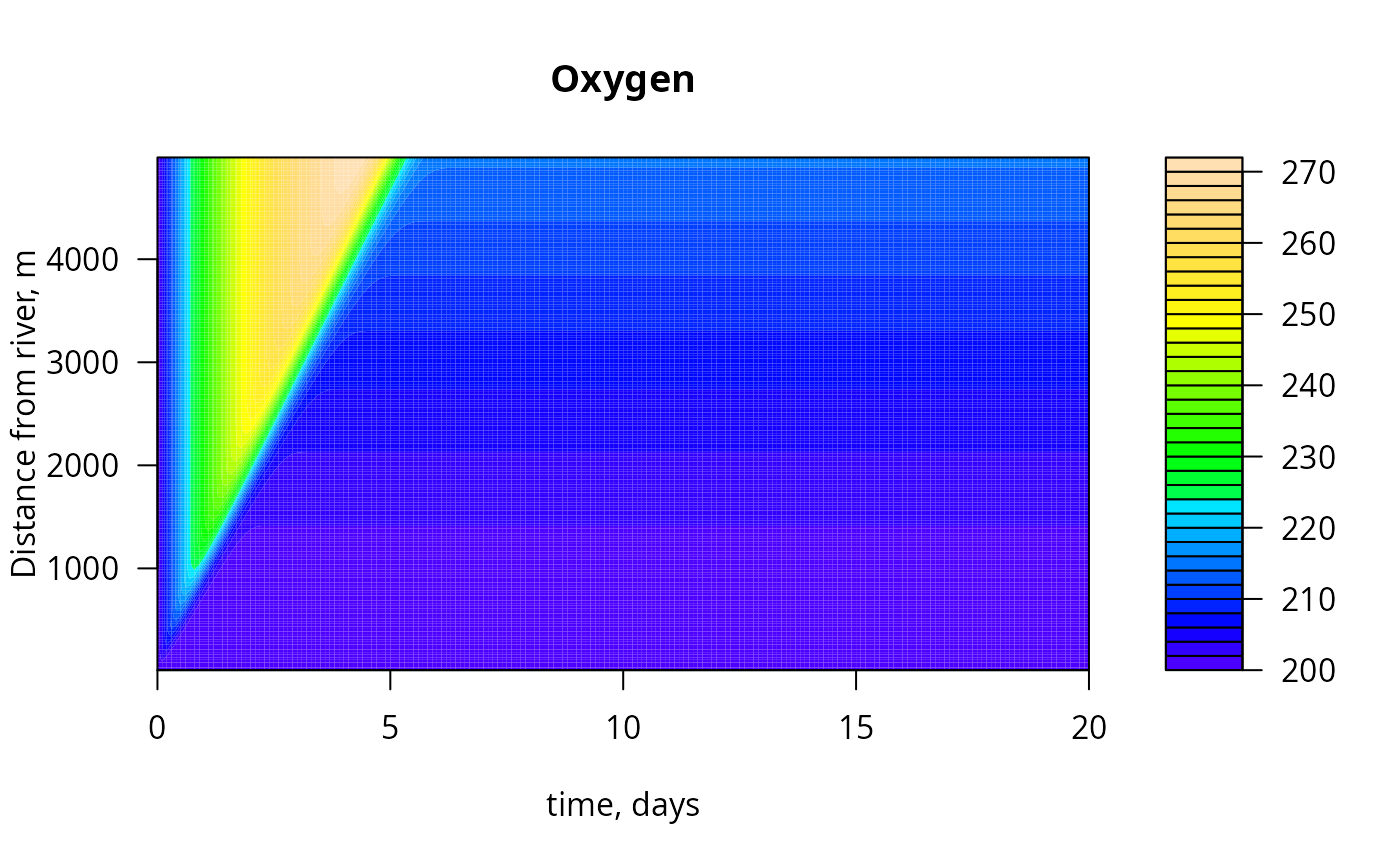
## ================
## Plotting output
## ================
## select oxygen (first column of out:time, then BOD, then O2
O2 <- out[, (N + 2):(2 * N + 1)]
color = topo.colors
filled.contour(x = times, y = x, O2, color = color, nlevels = 50,
xlab = "time, days", ylab = "Distance from river, m",
main = "Oxygen")
## =======================================================================
## Example 2.
## Biochemical Oxygen Demand (BOD) and oxygen (O2) dynamics
## in a river
## =======================================================================
## ================
## Model equations
## ================
O2BOD <- function(t, state, pars) {
BOD <- state[1:N]
O2 <- state[(N+1):(2*N)]
## BOD dynamics
FluxBOD <- v * c(BOD_0, BOD) # fluxes due to water transport
FluxO2 <- v * c(O2_0, O2)
BODrate <- r * BOD # 1-st order consumption
## rate of change = flux gradient - consumption + reaeration (O2)
dBOD <- -diff(FluxBOD)/dx - BODrate
dO2 <- -diff(FluxO2)/dx - BODrate + p * (O2sat-O2)
return(list(c(dBOD = dBOD, dO2 = dO2)))
}
## ==================
## Model application
## ==================
## parameters
dx <- 25 # grid size of 25 meters
v <- 1e3 # velocity, m/day
x <- seq(dx/2, 5000, by = dx) # m, distance from river
N <- length(x)
r <- 0.05 # /day, first-order decay of BOD
p <- 0.5 # /day, air-sea exchange rate
O2sat <- 300 # mmol/m3 saturated oxygen conc
O2_0 <- 200 # mmol/m3 riverine oxygen conc
BOD_0 <- 1000 # mmol/m3 riverine BOD concentration
## initial conditions:
state <- c(rep(200, N), rep(200, N))
times <- seq(0, 20, by = 0.1)
## running the model
## step 1 : model spinup
out <- ode.1D(y = state, times, O2BOD, parms = NULL,
nspec = 2, names = c("BOD", "O2"))
## ================
## Plotting output
## ================
## select oxygen (first column of out:time, then BOD, then O2
O2 <- out[, (N + 2):(2 * N + 1)]
color = topo.colors
filled.contour(x = times, y = x, O2, color = color, nlevels = 50,
xlab = "time, days", ylab = "Distance from river, m",
main = "Oxygen")
 ## or quicker plotting:
image(out, grid = x, xlab = "time, days", ylab = "Distance from river, m")
## or quicker plotting:
image(out, grid = x, xlab = "time, days", ylab = "Distance from river, m")