Plot, Image and Histogram Method for deSolve Objects
plot.deSolve.RdPlot the output of numeric integration routines.
Usage
# S3 method for class 'deSolve'
plot(x, ..., select = NULL, which = select, ask = NULL,
              obs = NULL, obspar = list(), subset = NULL)
<!-- %% thpe: since 1.14 not anymore exported -->
<!-- %\method{matplot}{deSolve}(x, \dots, select = NULL, which = select, -->
<!-- %              obs = NULL, obspar = list(), subset = NULL, -->
<!-- %              legend = list(x = "topright")) -->
# S3 method for class 'deSolve'
hist(x, select = 1:(ncol(x)-1), which  = select, ask = NULL,
              subset = NULL, ...)
# S3 method for class 'deSolve'
image(x, select = NULL, which = select, ask = NULL,
              add.contour = FALSE, grid = NULL,
              method = "image", legend = FALSE, subset = NULL, ...)
# S3 method for class 'deSolve'
subset(x, subset = NULL, select = NULL,
             which = select, arr = FALSE, ...)

plot.1D (x, ..., select = NULL, which = select, ask = NULL,
         obs = NULL, obspar = list(), grid = NULL,
         xyswap = FALSE, delay = 0, vertical = FALSE, subset = NULL)

matplot.0D(x, ..., select = NULL, which = select,
           obs = NULL, obspar = list(), subset = NULL,
           legend = list(x = "topright"))

matplot.1D(x, select = NULL, which = select, ask = NULL,
         obs = NULL, obspar = list(), grid = NULL,
         xyswap = FALSE, vertical = FALSE, subset = NULL, ...)
Arguments
- x
an object of class
deSolve, as returned by the integrators, and to be plotted.For
plot.deSolve, it is allowed to pass several objects of classdeSolveafterx(unnamed) - see second example.- which
the name(s) or the index to the variables that should be plotted or selected. Default = all variables, except
time. For use withmatplot.0Dandmatplot.1D,whichorselectcan be a list, with vectors, each referring to a separate y-axis.- select
which variable/columns to be selected. This is added for consistency with the R-function
subset.- subset
either a logical expression indicating elements or rows to keep in
select, or a vector of integers denoting the indices of the elements over which to loop. Missing values are taken asFALSE- ask
logical; if
TRUE, the user is asked before each plot, ifNULLthe user is only asked if more than one page of plots is necessary and the current graphics device is set interactive, seepar(ask)anddev.interactive.- add.contour
if
TRUE, will add contours to the image plot.- method
the name of the plotting method to use, one of "image", "filled.contour", "persp", "contour".
- grid
only for
imageplots and forplot.1D: the 1-D grid as a vector (for output generated withode.1D), or the x- and y-grid, as alist(for output generated withode.2D).- xyswap
if
TRUE, then x-and y-values are swapped and the y-axis is from top to bottom. Useful for drawing vertical profiles.- vertical
if
TRUE, then 1. x-and y-values are swapped, the y-axis is from top to bottom, the x-axis is on top, margin 3 and the main title gets the value of the x-axis. Useful for drawing vertical profiles; see example 2.- delay
adds a delay (in milliseconds) between consecutive plots of
plot.1Dto enable animations.- obs
a
data.frameormatrixwith "observed data" that will be added aspointsto the plots.obscan also be alistwith multiple data.frames and/or matrices containing observed data.By default the first column of an observed data set should contain the
time-variable. The other columns contain the observed values and they should have names that are known inx.If the first column of
obsconsists of factors or characters (strings), then it is assumed that the data are presented in long (database) format, where the first three columns contain (name, time, value).If
obsis notNULLandwhichisNULL, then the variables, common to bothobsandxwill be plotted.- obspar
additional graphics arguments passed to
points, for plotting the observed data. Ifobsis alistcontaining multiple observed data sets, then the graphics arguments can be a vector or a list (e.g. forxlim,ylim), specifying each data set separately.- legend
if
TRUE, a color legend will be drawn on the right of each image. For use withmatplot.0Dandmatplot.1D: alistwith arguments passed to R-function legend.- arr
if
TRUE, and the output is from a 2-D or 3-D model, an array will be returned with dimension = c(dimension of selected variable, nrow(x)). Whenarr=TRUEthen only one variable can be selected. When the output is from a 0-D or 1-D model, then this argument is ignored.- ...
additional arguments.
The graphical arguments are passed to
plot.default,imageorhistFor
plot.deSolve, andplot.1D, the dots may contain other objects of classdeSolve, as returned by the integrators, and to be plotted on the same graphs asx- see second example. In this case,xand and these other objects should be compatible, i.e. the column names should be the same.For
plot.deSolve, the arguments after ... must be matched exactly.
Value
Function subset called with arr = FALSE will return a
matrix with up to as many rows as selected by subset and as
many columns as selected variables.
When arr = TRUE then an array will be outputted with dimensions
equal to the dimension of the selected variable, augmented with the number
of rows selected by subset. This means that the last dimension points
to times.
Function subset also has an attribute that contains the times
selected.
Details
The number of panels per page is automatically determined up to 3 x 3
(par(mfrow = c(3, 3))). This default can be overwritten by
specifying user-defined settings for mfrow or mfcol.
Set mfrow equal to NULL to avoid the plotting function to
change user-defined mfrow or mfcol settings.
Other graphical parameters can be passed as well. Parameters are
vectorized, either according to the number of plots (xlab,
ylab, main, sub, xlim, ylim,
log, asp, ann, axes, frame.plot,
panel.first, panel.last, cex.lab,
cex.axis, cex.main) or according to the number of lines
within one plot (other parameters e.g. col, lty,
lwd etc.) so it is possible to assign specific axis labels to
individual plots, resp. different plotting style. Plotting parameter
ylim, or xlim can also be a list to assign different
axis limits to individual plots.
Similarly, the graphical parameters for observed data, as passed by
obspar can be vectorized, according to the number of observed
data sets.
Image plots will only work for 1-D and 2-D variables, as solved with
ode.1D and ode.2D. In the first case, an
image with times as x- and the grid as y-axis will be
created. In the second case, an x-y plot will be created, for all
times. Unless ask = FALSE, the user will be asked to confirm
page changes. Via argument mtext, it is possible to label each
page in case of 2D output.
For images, it is possible to pass an argument
method which can take the values "image" (default),
"filled.contour", "contour" or "persp", in order to use the respective
plotting method.
plot and matplot.0D will always have times on the x-axis.
For problems solved with ode.1D, it may be more useful to use
plot.1D or matplot.1D
which will plot how spatial variables change with time. These plots will
have the grid on the x-axis.
Examples
## =======================================================================
## Example 1. A Predator-Prey model with 4 species in matrix formulation
## =======================================================================
LVmatrix <- function(t, n, parms) {
with(parms, {
dn <- r * n + n * (A %*% n)
return(list(c(dn)))
})
}
parms <- list(
r = c(r1 = 0.1, r2 = 0.1, r3 = -0.1, r4 = -0.1),
A = matrix(c(0.0, 0.0, -0.2, 0.01, # prey 1
0.0, 0.0, 0.02, -0.1, # prey 2
0.2, 0.02, 0.0, 0.0, # predator 1; prefers prey 1
0.01, 0.1, 0.0, 0.0), # predator 2; prefers prey 2
nrow = 4, ncol = 4, byrow=TRUE)
)
times <- seq(from = 0, to = 500, by = 0.1)
y <- c(prey1 = 1, prey2 = 1, pred1 = 2, pred2 = 2)
out <- ode(y, times, LVmatrix, parms)
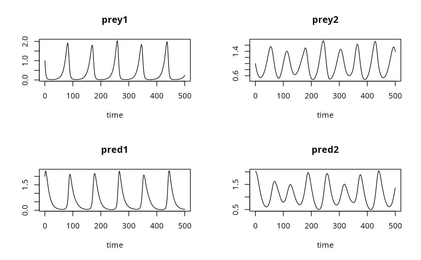
## Basic line plot
plot(out, type = "l")
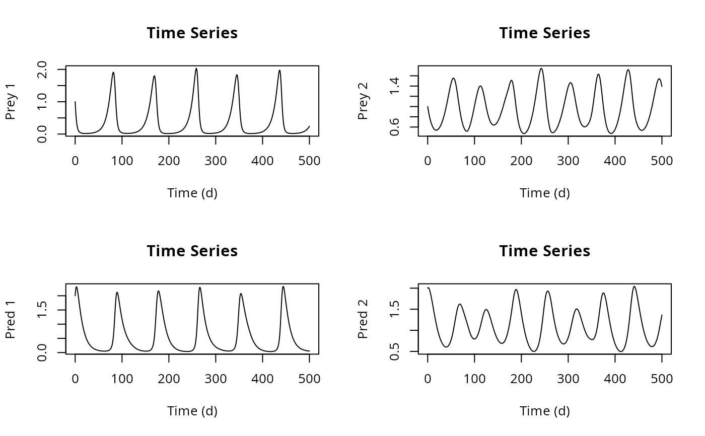
 ## User-specified axis labels
plot(out, type = "l", ylab = c("Prey 1", "Prey 2", "Pred 1", "Pred 2"),
xlab = "Time (d)", main = "Time Series")
## User-specified axis labels
plot(out, type = "l", ylab = c("Prey 1", "Prey 2", "Pred 1", "Pred 2"),
xlab = "Time (d)", main = "Time Series")
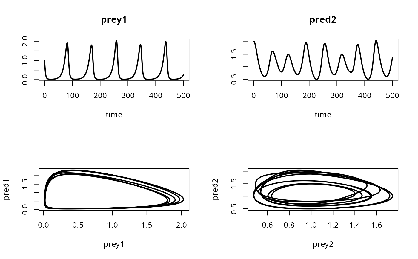
 ## Set user-defined mfrow
pm <- par (mfrow = c(2, 2))
## "mfrow=NULL" keeps user-defined mfrow
plot(out, which = c("prey1", "pred2"), mfrow = NULL, type = "l", lwd = 2)
plot(out[,"prey1"], out[,"pred1"], xlab="prey1",
ylab = "pred1", type = "l", lwd = 2)
plot(out[,"prey2"], out[,"pred2"], xlab = "prey2",
ylab = "pred2", type = "l",lwd = 2)
## Set user-defined mfrow
pm <- par (mfrow = c(2, 2))
## "mfrow=NULL" keeps user-defined mfrow
plot(out, which = c("prey1", "pred2"), mfrow = NULL, type = "l", lwd = 2)
plot(out[,"prey1"], out[,"pred1"], xlab="prey1",
ylab = "pred1", type = "l", lwd = 2)
plot(out[,"prey2"], out[,"pred2"], xlab = "prey2",
ylab = "pred2", type = "l",lwd = 2)
 ## restore graphics parameters
par ("mfrow" = pm)
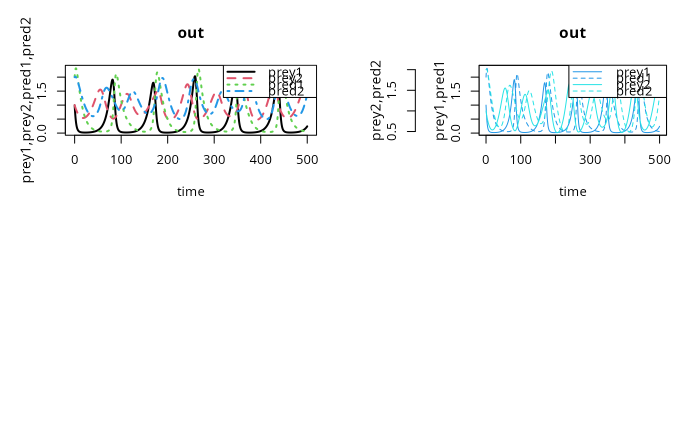
## Plot all in one figure, using matplot
matplot.0D(out, lwd = 2)
## Split y-variables in two groups
matplot.0D(out, which = list(c(1,3), c(2,4)),
lty = c(1,2,1,2), col=c(4,4,5,5),
ylab = c("prey1,pred1", "prey2,pred2"))
## =======================================================================
## Example 2. Add second and third output, and observations
## =======================================================================
# New runs with different parameter settings
parms2 <- parms
parms2$r[1] <- 0.2
out2 <- ode(y, times, LVmatrix, parms2)
# New runs with different parameter settings
parms3 <- parms
parms3$r[1] <- 0.05
out3 <- ode(y, times, LVmatrix, parms3)
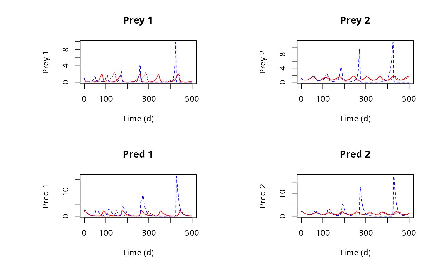
# plot all three outputs
plot(out, out2, out3, type = "l",
ylab = c("Prey 1", "Prey 2", "Pred 1", "Pred 2"),
xlab = "Time (d)", main = c("Prey 1", "Prey 2", "Pred 1", "Pred 2"),
col = c("red", "blue", "darkred"))
## restore graphics parameters
par ("mfrow" = pm)
## Plot all in one figure, using matplot
matplot.0D(out, lwd = 2)
## Split y-variables in two groups
matplot.0D(out, which = list(c(1,3), c(2,4)),
lty = c(1,2,1,2), col=c(4,4,5,5),
ylab = c("prey1,pred1", "prey2,pred2"))
## =======================================================================
## Example 2. Add second and third output, and observations
## =======================================================================
# New runs with different parameter settings
parms2 <- parms
parms2$r[1] <- 0.2
out2 <- ode(y, times, LVmatrix, parms2)
# New runs with different parameter settings
parms3 <- parms
parms3$r[1] <- 0.05
out3 <- ode(y, times, LVmatrix, parms3)
# plot all three outputs
plot(out, out2, out3, type = "l",
ylab = c("Prey 1", "Prey 2", "Pred 1", "Pred 2"),
xlab = "Time (d)", main = c("Prey 1", "Prey 2", "Pred 1", "Pred 2"),
col = c("red", "blue", "darkred"))
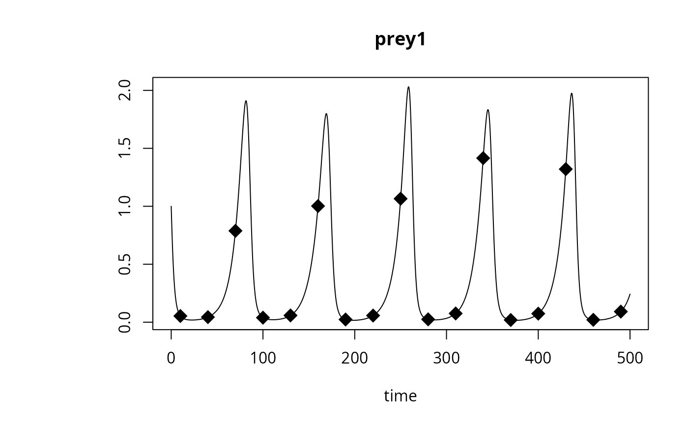
 ## 'observed' data
obs <- as.data.frame(out[out[,1] %in% seq(10, 500, by = 30), ])
plot(out, which = "prey1", type = "l", obs = obs,
obspar = list(pch = 18, cex = 2))
## 'observed' data
obs <- as.data.frame(out[out[,1] %in% seq(10, 500, by = 30), ])
plot(out, which = "prey1", type = "l", obs = obs,
obspar = list(pch = 18, cex = 2))
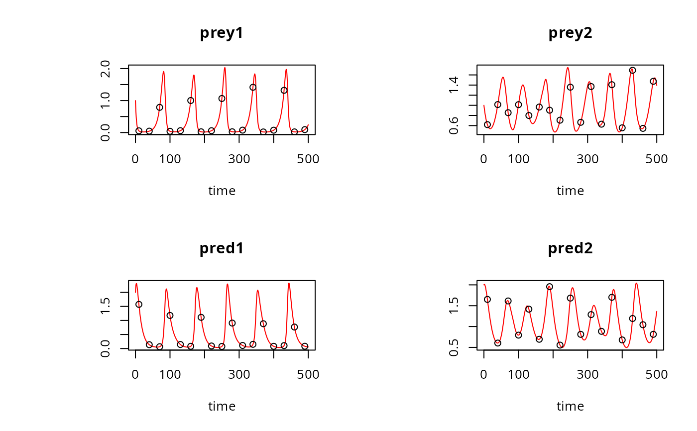
 plot(out, type = "l", obs = obs, col = "red")
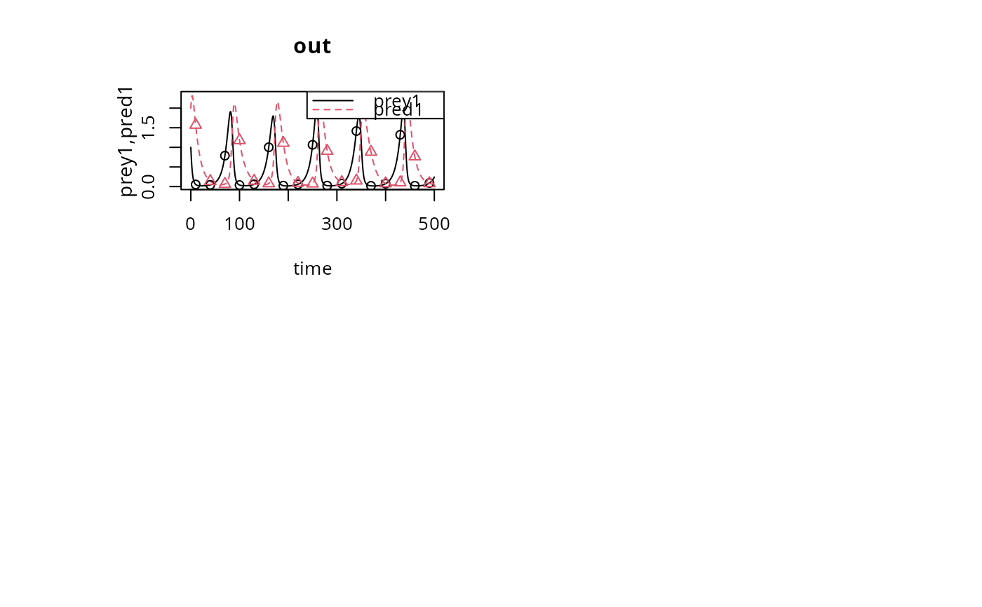
 matplot.0D(out, which = c("prey1", "pred1"), type = "l", obs = obs)
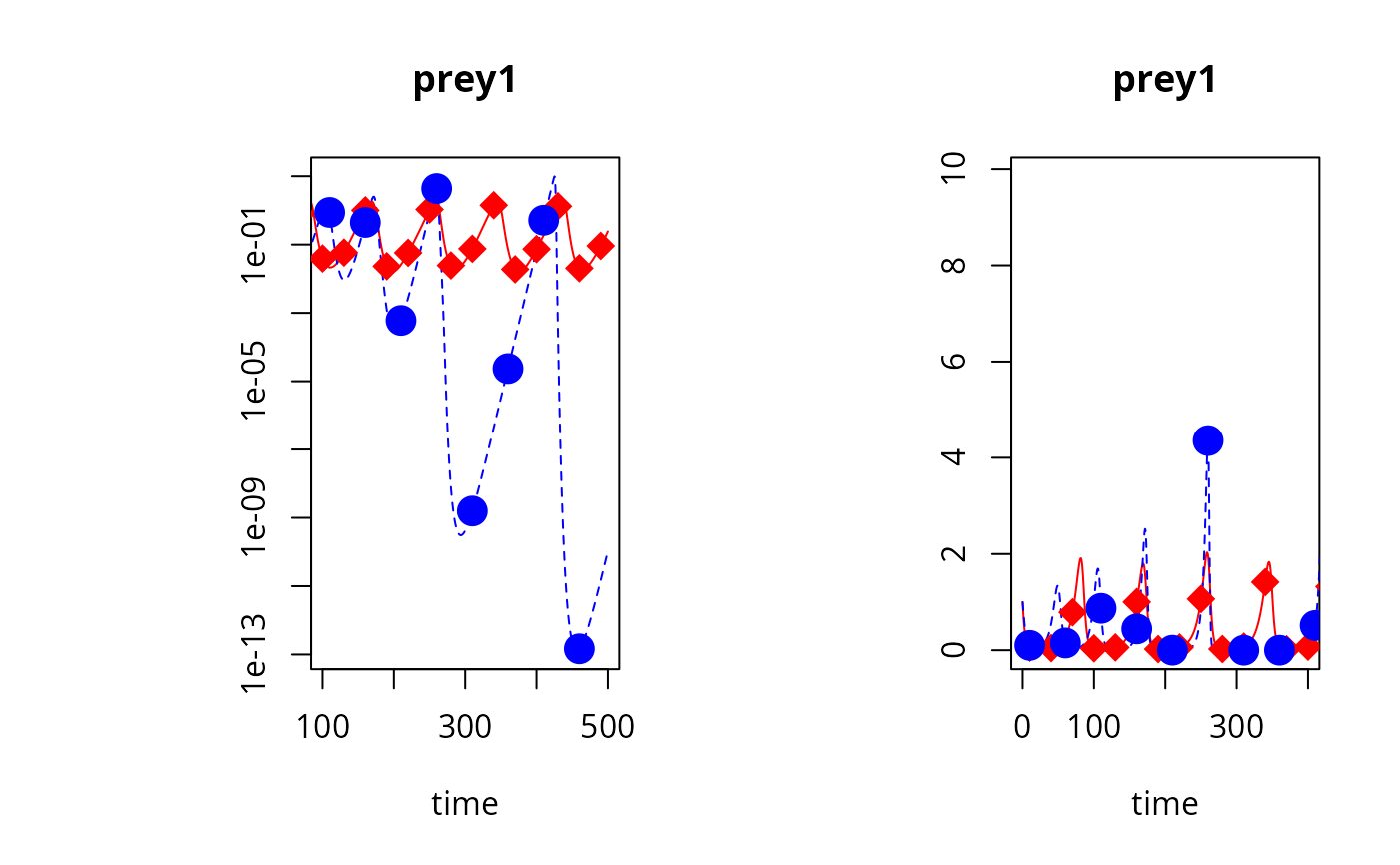
## second set of 'observed' data and two outputs
obs2 <- as.data.frame(out2[out2[,1] %in% seq(10, 500, by = 50), ])
## manual xlim, log
plot(out, out2, type = "l", obs = list(obs, obs2), col = c("red", "blue"),
obspar = list(pch = 18:19, cex = 2, col = c("red", "blue")),
log = c("y", ""), which = c("prey1", "prey1"),
xlim = list(c(100, 500), c(0, 400)))
matplot.0D(out, which = c("prey1", "pred1"), type = "l", obs = obs)
## second set of 'observed' data and two outputs
obs2 <- as.data.frame(out2[out2[,1] %in% seq(10, 500, by = 50), ])
## manual xlim, log
plot(out, out2, type = "l", obs = list(obs, obs2), col = c("red", "blue"),
obspar = list(pch = 18:19, cex = 2, col = c("red", "blue")),
log = c("y", ""), which = c("prey1", "prey1"),
xlim = list(c(100, 500), c(0, 400)))
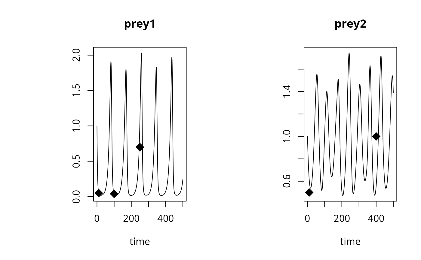
 ## data in 'long' format
OBS <- data.frame(name = c(rep("prey1", 3), rep("prey2", 2)),
time = c(10, 100, 250, 10, 400),
value = c(0.05, 0.04, 0.7, 0.5, 1))
OBS
#> name time value
#> 1 prey1 10 0.05
#> 2 prey1 100 0.04
#> 3 prey1 250 0.70
#> 4 prey2 10 0.50
#> 5 prey2 400 1.00
plot(out, obs = OBS, obspar = c(pch = 18, cex = 2))
## data in 'long' format
OBS <- data.frame(name = c(rep("prey1", 3), rep("prey2", 2)),
time = c(10, 100, 250, 10, 400),
value = c(0.05, 0.04, 0.7, 0.5, 1))
OBS
#> name time value
#> 1 prey1 10 0.05
#> 2 prey1 100 0.04
#> 3 prey1 250 0.70
#> 4 prey2 10 0.50
#> 5 prey2 400 1.00
plot(out, obs = OBS, obspar = c(pch = 18, cex = 2))
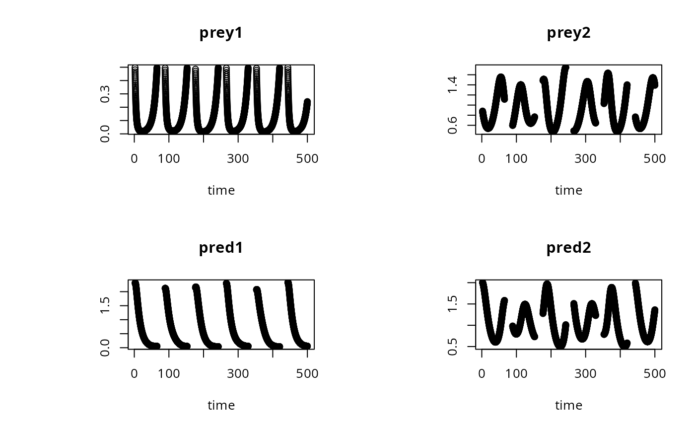
 # a subset only:
plot(out, subset = prey1 < 0.5, type = "p")
# a subset only:
plot(out, subset = prey1 < 0.5, type = "p")
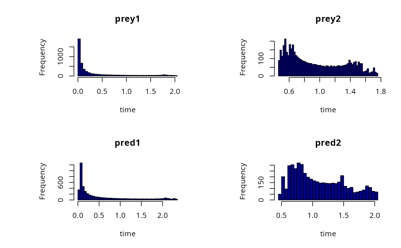
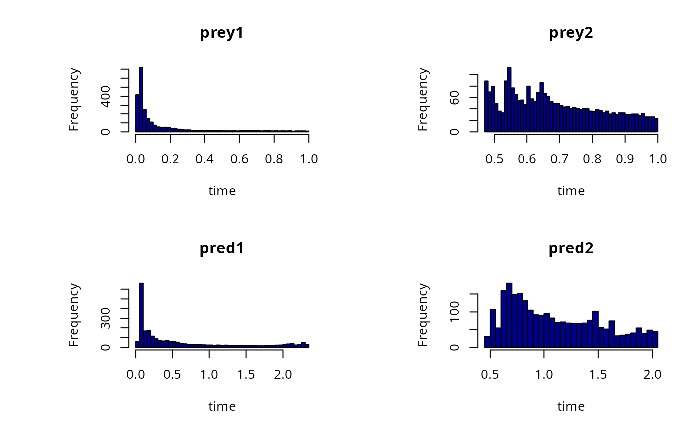
 # Simple histogram
hist(out, col = "darkblue", breaks = 50)
# Simple histogram
hist(out, col = "darkblue", breaks = 50)
 hist(out, col = "darkblue", breaks = 50, subset = prey1<1 & prey2 < 1)
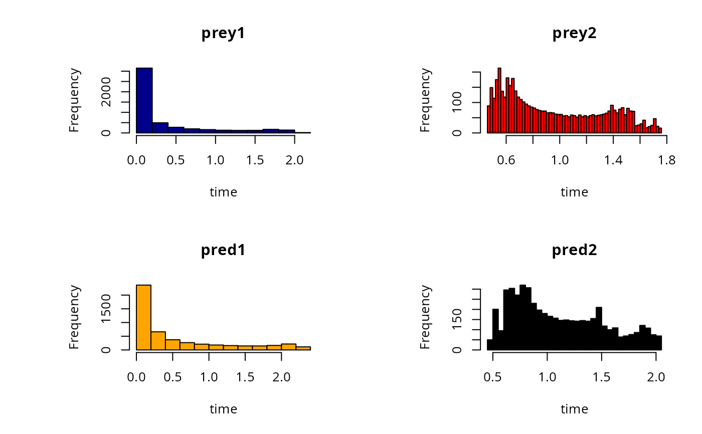
 # different parameters per plot
hist(out, col = c("darkblue", "red", "orange", "black"),
breaks = c(10,50))
# different parameters per plot
hist(out, col = c("darkblue", "red", "orange", "black"),
breaks = c(10,50))
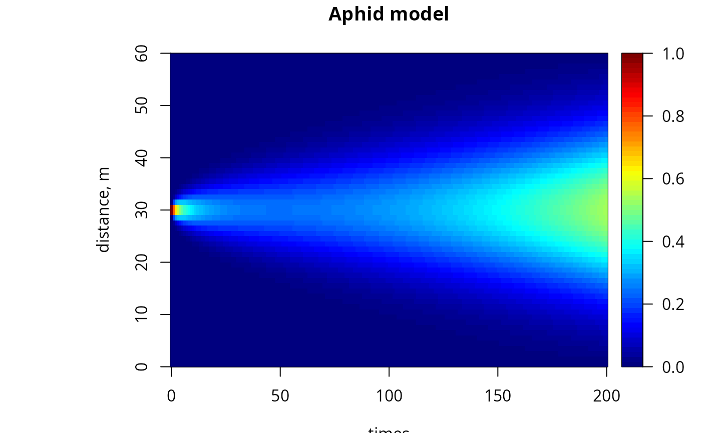
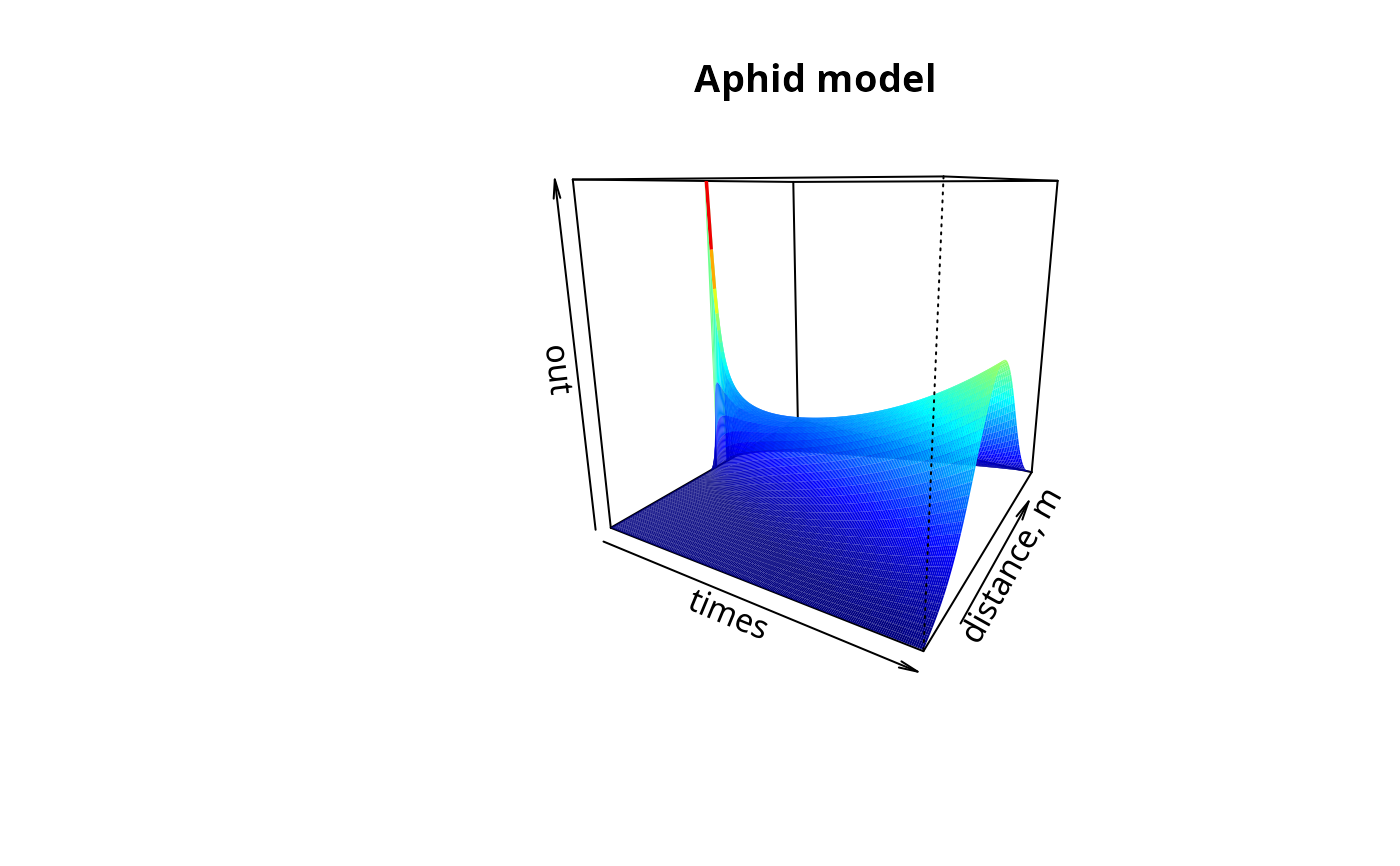
 ## =======================================================================
## The Aphid model from Soetaert and Herman, 2009.
## A practical guide to ecological modelling.
## Using R as a simulation platform. Springer.
## =======================================================================
## 1-D diffusion model
## ================
## Model equations
## ================
Aphid <- function(t, APHIDS, parameters) {
deltax <- c (0.5*delx, rep(delx, numboxes - 1), 0.5*delx)
Flux <- -D * diff(c(0, APHIDS, 0))/deltax
dAPHIDS <- -diff(Flux)/delx + APHIDS * r
list(dAPHIDS, Flux = Flux)
}
## ==================
## Model application
## ==================
## the model parameters:
D <- 0.3 # m2/day diffusion rate
r <- 0.01 # /day net growth rate
delx <- 1 # m thickness of boxes
numboxes <- 60
## distance of boxes on plant, m, 1 m intervals
Distance <- seq(from = 0.5, by = delx, length.out = numboxes)
## Initial conditions, ind/m2
## aphids present only on two central boxes
APHIDS <- rep(0, times = numboxes)
APHIDS[30:31] <- 1
state <- c(APHIDS = APHIDS) # initialise state variables
## RUNNING the model:
times <- seq(0, 200, by = 1) # output wanted at these time intervals
out <- ode.1D(state, times, Aphid, parms = 0, nspec = 1, names = "Aphid")
image(out, grid = Distance, main = "Aphid model", ylab = "distance, m",
legend = TRUE)
## =======================================================================
## The Aphid model from Soetaert and Herman, 2009.
## A practical guide to ecological modelling.
## Using R as a simulation platform. Springer.
## =======================================================================
## 1-D diffusion model
## ================
## Model equations
## ================
Aphid <- function(t, APHIDS, parameters) {
deltax <- c (0.5*delx, rep(delx, numboxes - 1), 0.5*delx)
Flux <- -D * diff(c(0, APHIDS, 0))/deltax
dAPHIDS <- -diff(Flux)/delx + APHIDS * r
list(dAPHIDS, Flux = Flux)
}
## ==================
## Model application
## ==================
## the model parameters:
D <- 0.3 # m2/day diffusion rate
r <- 0.01 # /day net growth rate
delx <- 1 # m thickness of boxes
numboxes <- 60
## distance of boxes on plant, m, 1 m intervals
Distance <- seq(from = 0.5, by = delx, length.out = numboxes)
## Initial conditions, ind/m2
## aphids present only on two central boxes
APHIDS <- rep(0, times = numboxes)
APHIDS[30:31] <- 1
state <- c(APHIDS = APHIDS) # initialise state variables
## RUNNING the model:
times <- seq(0, 200, by = 1) # output wanted at these time intervals
out <- ode.1D(state, times, Aphid, parms = 0, nspec = 1, names = "Aphid")
image(out, grid = Distance, main = "Aphid model", ylab = "distance, m",
legend = TRUE)
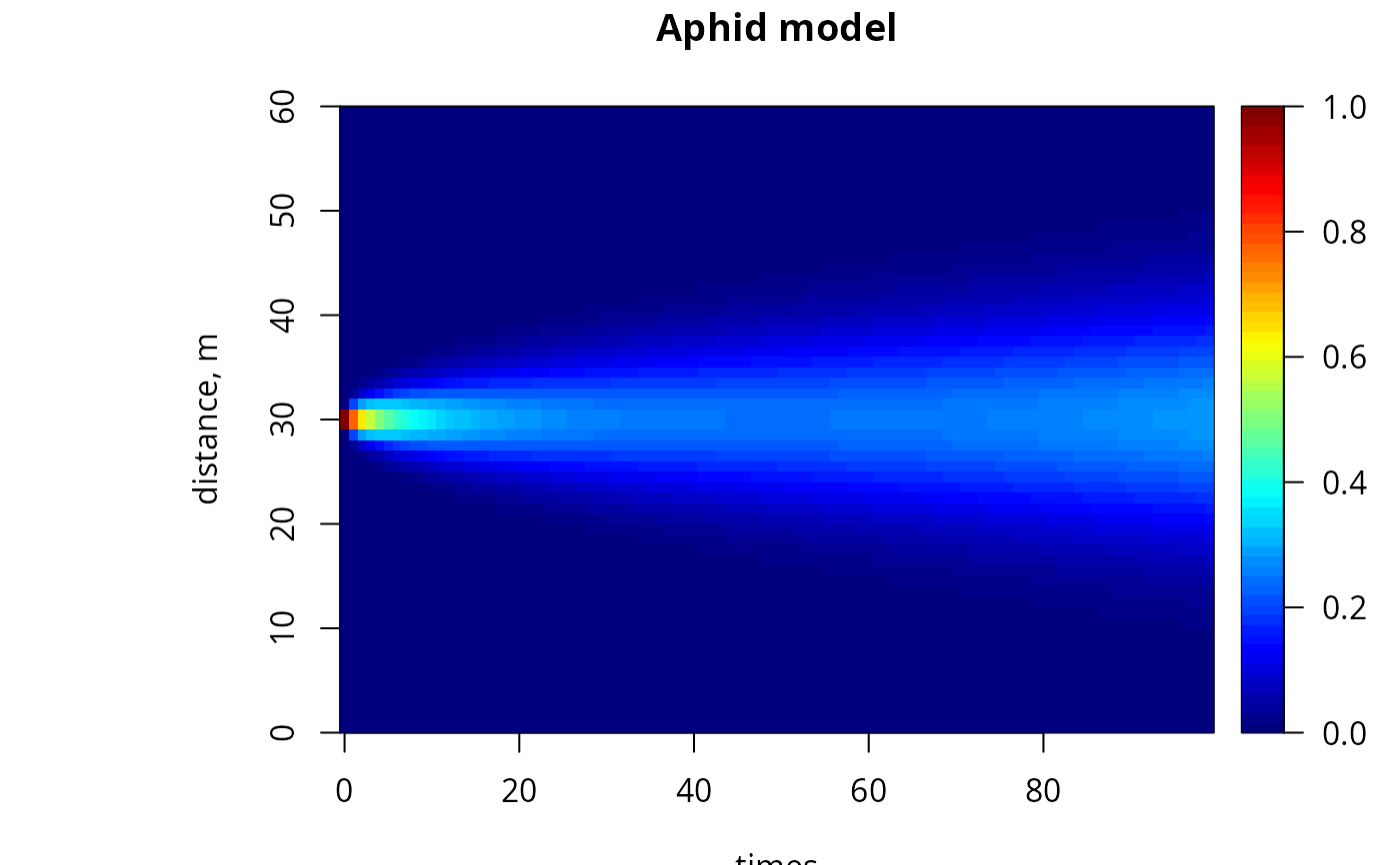
 ## restricting time
image(out, grid = Distance, main = "Aphid model", ylab = "distance, m",
legend = TRUE, subset = time < 100)
## restricting time
image(out, grid = Distance, main = "Aphid model", ylab = "distance, m",
legend = TRUE, subset = time < 100)
 image(out, grid = Distance, main = "Aphid model", ylab = "distance, m",
method = "persp", border = NA, theta = 30)
image(out, grid = Distance, main = "Aphid model", ylab = "distance, m",
method = "persp", border = NA, theta = 30)
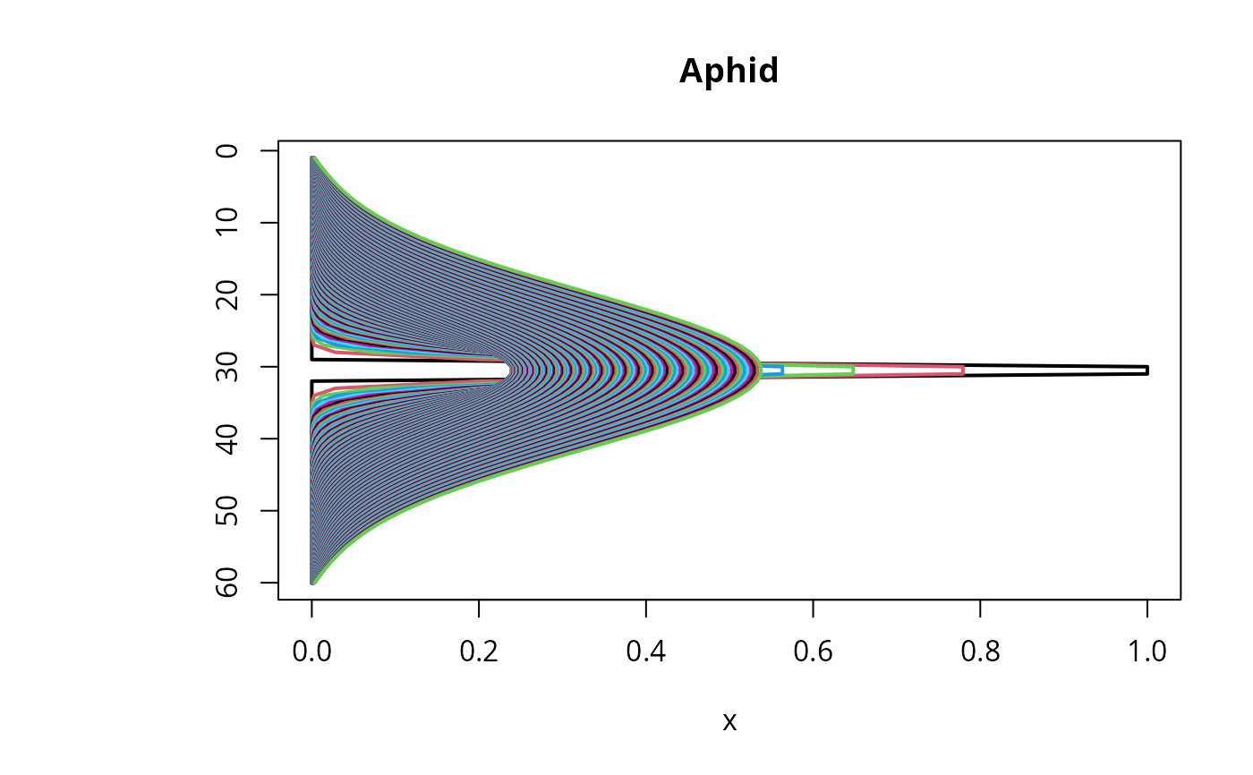
 FluxAphid <- subset(out, select = "Flux", subset = time < 50)
matplot.1D(out, type = "l", lwd = 2, xyswap = TRUE, lty = 1)
FluxAphid <- subset(out, select = "Flux", subset = time < 50)
matplot.1D(out, type = "l", lwd = 2, xyswap = TRUE, lty = 1)
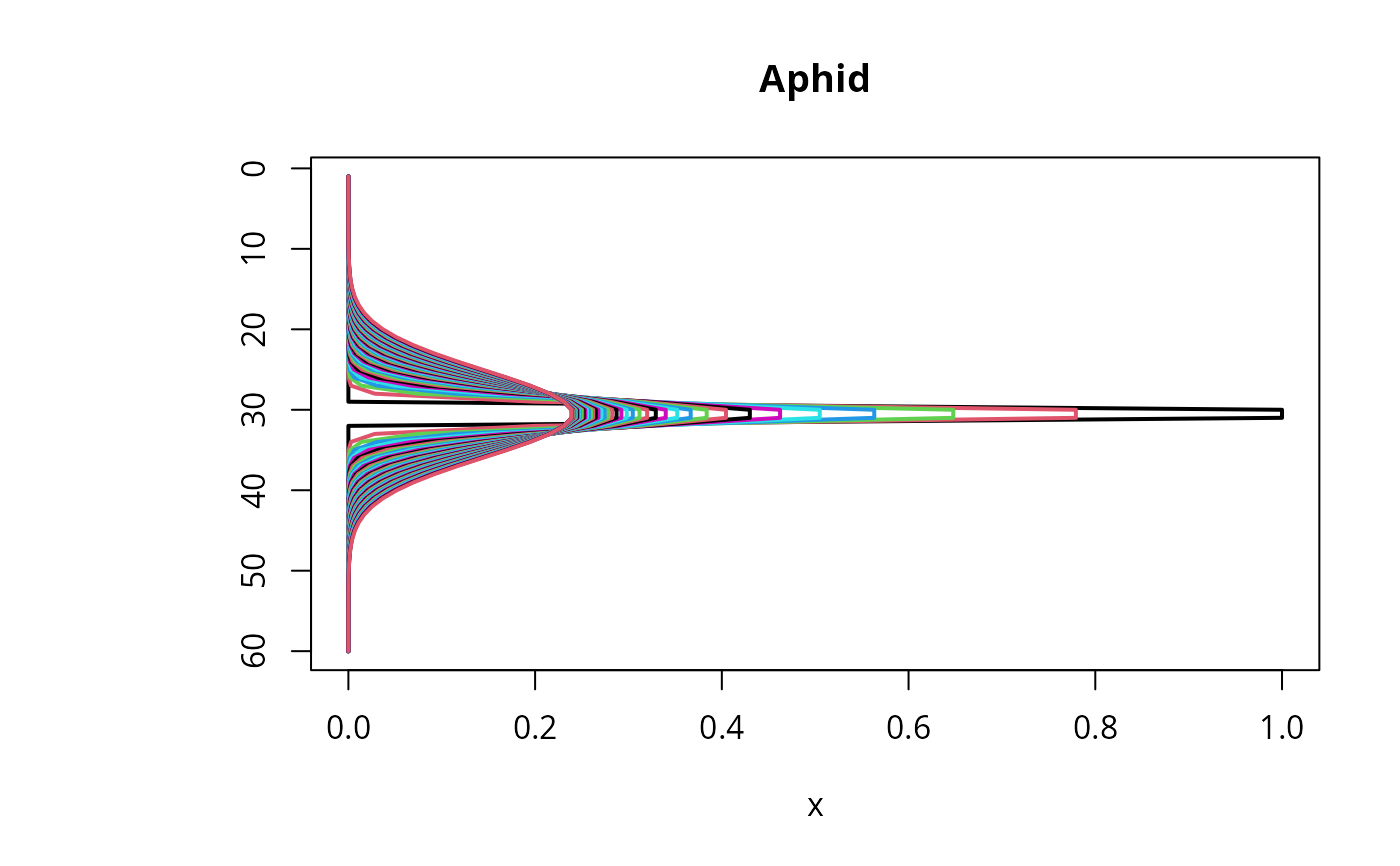
 matplot.1D(out, type = "l", lwd = 2, xyswap = TRUE, lty = 1,
subset = time < 50)
matplot.1D(out, type = "l", lwd = 2, xyswap = TRUE, lty = 1,
subset = time < 50)
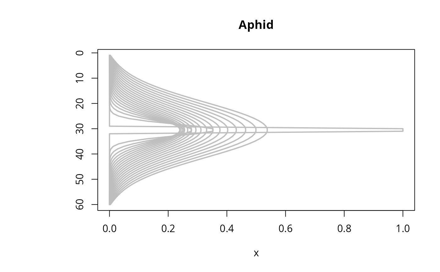
 matplot.1D(out, type = "l", lwd = 2, xyswap = TRUE, lty = 1,
subset = time %in% seq(0, 200, by = 10), col = "grey")
matplot.1D(out, type = "l", lwd = 2, xyswap = TRUE, lty = 1,
subset = time %in% seq(0, 200, by = 10), col = "grey")
 if (FALSE) { # \dontrun{
plot(out, ask = FALSE, mfrow = c(1, 1))
plot.1D(out, ask = FALSE, type = "l", lwd = 2, xyswap = TRUE)
} # }
## see help file for ode.2D for images of 2D variables
if (FALSE) { # \dontrun{
plot(out, ask = FALSE, mfrow = c(1, 1))
plot.1D(out, ask = FALSE, type = "l", lwd = 2, xyswap = TRUE)
} # }
## see help file for ode.2D for images of 2D variables