Solver for 2-Dimensional Ordinary Differential Equations
ode.2D.RdSolves a system of ordinary differential equations resulting from 2-Dimensional partial differential equations that have been converted to ODEs by numerical differencing.
Usage
ode.2D(y, times, func, parms, nspec = NULL, dimens,
  method= c("lsodes", "euler", "rk4", "ode23", "ode45", "adams", "iteration"),
  names = NULL, cyclicBnd = NULL, ...)
Arguments
- y
the initial (state) values for the ODE system, a vector. If
yhas a name attribute, the names will be used to label the output matrix.- times
time sequence for which output is wanted; the first value of
timesmust be the initial time.- func
either an R-function that computes the values of the derivatives in the ODE system (the model definition) at time
t, or a character string giving the name of a compiled function in a dynamically loaded shared library.If
funcis an R-function, it must be defined as:func <- function(t, y, parms, ...).tis the current time point in the integration,yis the current estimate of the variables in the ODE system. If the initial valuesyhas anamesattribute, the names will be available insidefunc.parmsis a vector or list of parameters;...(optional) are any other arguments passed to the function.The return value of
funcshould be a list, whose first element is a vector containing the derivatives ofywith respect totime, and whose next elements are global values that are required at each point intimes. The derivatives must be specified in the same order as the state variablesy.- parms
parameters passed to
func.- nspec
the number of species (components) in the model.
- dimens
2-valued vector with the number of boxes in two dimensions in the model.
- cyclicBnd
if not
NULLthen a number or a 2-valued vector with the dimensions where a cyclic boundary is used -1: x-dimension,2: y-dimension; see details.- names
the names of the components; used for plotting.
- method
the integrator. Use
"lsodes"if the model is very stiff;"impAdams"may be best suited for mildly stiff problems;"euler", "rk4", "ode23", "ode45", "adams"are most efficient for non-stiff problems. Also allowed is to pass an integratorfunction. Use one of the other Runge-Kutta methods viarkMethod. For instance,method = rkMethod("ode45ck")will trigger the Cash-Karp method of order 4(5).If
"lsodes"is used, then also the size of the work array should be specified (lrw) (see lsodes).Method
"iteration"is special in that here the functionfuncshould return the new value of the state variables rather than the rate of change. This can be used for individual based models, for difference equations, or in those cases where the integration is performed withinfunc)- ...
additional arguments passed to
lsodes.
Value
A matrix of class deSolve with up to as many rows as elements in times and as many
columns as elements in y plus the number of "global" values
returned in the second element of the return from func, plus an
additional column (the first) for the time value. There will be one
row for each element in times unless the integrator returns
with an unrecoverable error. If y has a names attribute, it
will be used to label the columns of the output value.
The output will have the attributes istate, and rstate,
two vectors with several useful elements. The first element of istate
returns the conditions under which the last call to the integrator
returned. Normal is istate = 2. If verbose = TRUE, the
settings of istate and rstate will be written to the screen. See the
help for the selected integrator for details.
Note
It is advisable though not mandatory to specify both
nspec and dimens. In this case, the solver can check
whether the input makes sense (as nspec * dimens[1] * dimens[2]
== length(y)).
Do not use this method for problems that are not 2D!
Details
This is the method of choice for 2-dimensional models, that are only subjected to transport between adjacent layers.
Based on the dimension of the problem, and if lsodes is used as
the integrator, the method first calculates the
sparsity pattern of the Jacobian, under the assumption that transport
is only occurring between adjacent layers. Then lsodes is
called to solve the problem.
If the model is not stiff, then it is more efficient to use one of the explicit integration routines
In some cases, a cyclic boundary condition exists. This is when the first
boxes in x-or y-direction interact with the last boxes. In this case, there
will be extra non-zero fringes in the Jacobian which need to be taken
into account. The occurrence of cyclic boundaries can be
toggled on by specifying argument cyclicBnd. For innstance,
cyclicBnd = 1 indicates that a cyclic boundary is required only for
the x-direction, whereas cyclicBnd = c(1,2) imposes a cyclic boundary
for both x- and y-direction. The default is no cyclic boundaries.
If lsodes is used to integrate, it will probably be necessary
to specify the length of the real work array, lrw.
Although a reasonable guess of lrw is made, it is likely that
this will be too low. In this case, ode.2D will return with an
error message telling the size of the work array actually needed. In
the second try then, set lrw equal to this number.
For instance, if you get the error:
DLSODES- RWORK length is insufficient to proceed.
  Length needed is .ge. LENRW (=I1), exceeds LRW (=I2)
  In above message,  I1 =     27627   I2 =     25932
set lrw equal to 27627 or a higher value.
See lsodes for the additional options.
Examples
## =======================================================================
## A Lotka-Volterra predator-prey model with predator and prey
## dispersing in 2 dimensions
## =======================================================================
## ==================
## Model definitions
## ==================
lvmod2D <- function (time, state, pars, N, Da, dx) {
NN <- N*N
Prey <- matrix(nrow = N, ncol = N,state[1:NN])
Pred <- matrix(nrow = N, ncol = N,state[(NN+1):(2*NN)])
with (as.list(pars), {
## Biology
dPrey <- rGrow * Prey * (1- Prey/K) - rIng * Prey * Pred
dPred <- rIng * Prey * Pred*assEff - rMort * Pred
zero <- rep(0, N)
## 1. Fluxes in x-direction; zero fluxes near boundaries
FluxPrey <- -Da * rbind(zero,(Prey[2:N,] - Prey[1:(N-1),]), zero)/dx
FluxPred <- -Da * rbind(zero,(Pred[2:N,] - Pred[1:(N-1),]), zero)/dx
## Add flux gradient to rate of change
dPrey <- dPrey - (FluxPrey[2:(N+1),] - FluxPrey[1:N,])/dx
dPred <- dPred - (FluxPred[2:(N+1),] - FluxPred[1:N,])/dx
## 2. Fluxes in y-direction; zero fluxes near boundaries
FluxPrey <- -Da * cbind(zero,(Prey[,2:N] - Prey[,1:(N-1)]), zero)/dx
FluxPred <- -Da * cbind(zero,(Pred[,2:N] - Pred[,1:(N-1)]), zero)/dx
## Add flux gradient to rate of change
dPrey <- dPrey - (FluxPrey[,2:(N+1)] - FluxPrey[,1:N])/dx
dPred <- dPred - (FluxPred[,2:(N+1)] - FluxPred[,1:N])/dx
return(list(c(as.vector(dPrey), as.vector(dPred))))
})
}
## ===================
## Model applications
## ===================
pars <- c(rIng = 0.2, # /day, rate of ingestion
rGrow = 1.0, # /day, growth rate of prey
rMort = 0.2 , # /day, mortality rate of predator
assEff = 0.5, # -, assimilation efficiency
K = 5 ) # mmol/m3, carrying capacity
R <- 20 # total length of surface, m
N <- 50 # number of boxes in one direction
dx <- R/N # thickness of each layer
Da <- 0.05 # m2/d, dispersion coefficient
NN <- N*N # total number of boxes
## initial conditions
yini <- rep(0, 2*N*N)
cc <- c((NN/2):(NN/2+1)+N/2, (NN/2):(NN/2+1)-N/2)
yini[cc] <- yini[NN+cc] <- 1
## solve model (5000 state variables... use Cash-Karp Runge-Kutta method
times <- seq(0, 50, by = 1)
out <- ode.2D(y = yini, times = times, func = lvmod2D, parms = pars,
dimens = c(N, N), names = c("Prey", "Pred"),
N = N, dx = dx, Da = Da, method = rkMethod("rk45ck"))
diagnostics(out)
#>
#> --------------------
#> rk return code
#> --------------------
#>
#> return code (idid) = 0
#> Integration was successful.
#>
#> --------------------
#> INTEGER values
#> --------------------
#>
#> 1 The return code : 0
#> 2 The number of steps taken for the problem so far: 74
#> 3 The number of function evaluations for the problem so far: 446
#> 13 The number of error test failures of the integrator so far: 1
#> 18 The order (or maximum order) of the method: 4
#>
summary(out)
#> Prey Pred
#> Min. -1.097020e-17 -1.601771e-19
#> 1st Qu. 2.454901e-05 1.524433e-12
#> Median 3.047291e+00 2.014444e-05
#> Mean 2.626324e+00 3.896581e-01
#> 3rd Qu. 4.936181e+00 8.264158e-02
#> Max. 4.999996e+00 3.119243e+00
#> N 1.275000e+05 1.275000e+05
#> sd 2.188556e+00 8.801305e-01
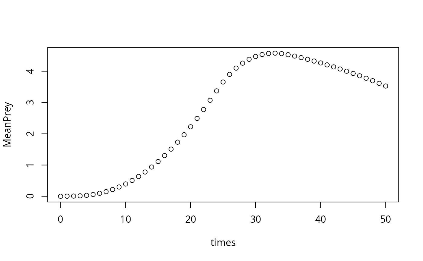
# Mean of prey concentration at each time step
Prey <- subset(out, select = "Prey", arr = TRUE)
dim(Prey)
#> [1] 50 50 51
MeanPrey <- apply(Prey, MARGIN = 3, FUN = mean)
plot(times, MeanPrey)
 if (FALSE) { # \dontrun{
## plot results
Col <- colorRampPalette(c("#00007F", "blue", "#007FFF", "cyan",
"#7FFF7F", "yellow", "#FF7F00", "red", "#7F0000"))
for (i in seq(1, length(times), by = 1))
image(Prey[ , ,i],
col = Col(100), xlab = , zlim = range(out[,2:(NN+1)]))
## similar, plotting both and adding a margin text with times:
image(out, xlab = "x", ylab = "y", mtext = paste("time = ", times))
} # }
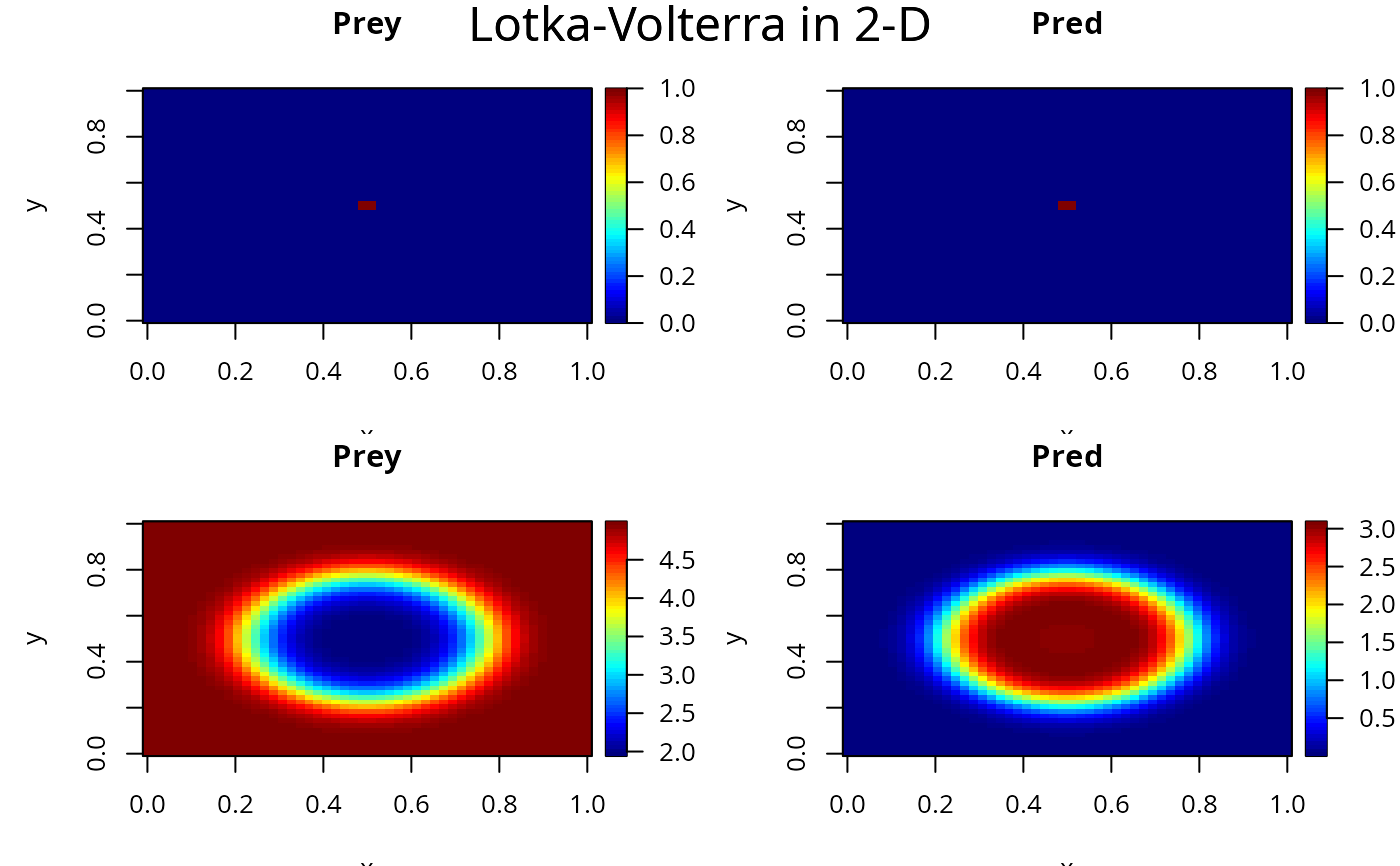
select <- c(1, 40)
image(out, xlab = "x", ylab = "y", mtext = "Lotka-Volterra in 2-D",
subset = select, mfrow = c(2,2), legend = TRUE)
if (FALSE) { # \dontrun{
## plot results
Col <- colorRampPalette(c("#00007F", "blue", "#007FFF", "cyan",
"#7FFF7F", "yellow", "#FF7F00", "red", "#7F0000"))
for (i in seq(1, length(times), by = 1))
image(Prey[ , ,i],
col = Col(100), xlab = , zlim = range(out[,2:(NN+1)]))
## similar, plotting both and adding a margin text with times:
image(out, xlab = "x", ylab = "y", mtext = paste("time = ", times))
} # }
select <- c(1, 40)
image(out, xlab = "x", ylab = "y", mtext = "Lotka-Volterra in 2-D",
subset = select, mfrow = c(2,2), legend = TRUE)
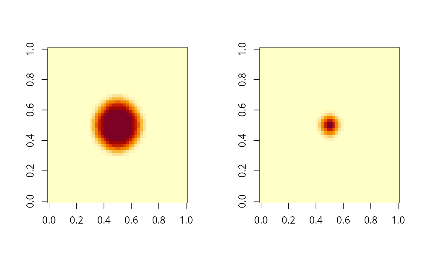
 # plot prey and pred at t = 10; first use subset to select data
prey10 <- matrix (nrow = N, ncol = N,
data = subset(out, select = "Prey", subset = (time == 10)))
pred10 <- matrix (nrow = N, ncol = N,
data = subset(out, select = "Pred", subset = (time == 10)))
mf <- par(mfrow = c(1, 2))
image(prey10)
image(pred10)
# plot prey and pred at t = 10; first use subset to select data
prey10 <- matrix (nrow = N, ncol = N,
data = subset(out, select = "Prey", subset = (time == 10)))
pred10 <- matrix (nrow = N, ncol = N,
data = subset(out, select = "Pred", subset = (time == 10)))
mf <- par(mfrow = c(1, 2))
image(prey10)
image(pred10)
 par (mfrow = mf)
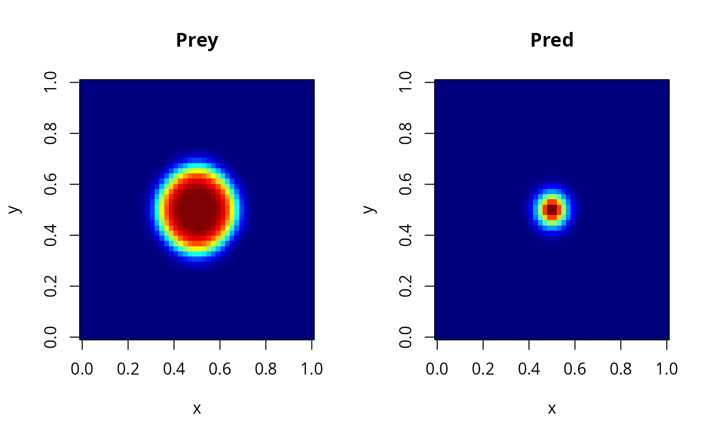
# same, using deSolve's image:
image(out, subset = (time == 10))
par (mfrow = mf)
# same, using deSolve's image:
image(out, subset = (time == 10))
 ## =======================================================================
## An example with a cyclic boundary condition.
## Diffusion in 2-D; extra flux on 2 boundaries,
## cyclic boundary in y
## =======================================================================
diffusion2D <- function(t, Y, par) {
y <- matrix(nrow = nx, ncol = ny, data = Y) # vector to 2-D matrix
dY <- -r * y # consumption
BNDx <- rep(1, nx) # boundary concentration
BNDy <- rep(1, ny) # boundary concentration
## diffusion in X-direction; boundaries=imposed concentration
Flux <- -Dx * rbind(y[1,] - BNDy, (y[2:nx,] - y[1:(nx-1),]), BNDy - y[nx,])/dx
dY <- dY - (Flux[2:(nx+1),] - Flux[1:nx,])/dx
## diffusion in Y-direction
Flux <- -Dy * cbind(y[,1] - BNDx, (y[,2:ny]-y[,1:(ny-1)]), BNDx - y[,ny])/dy
dY <- dY - (Flux[,2:(ny+1)] - Flux[,1:ny])/dy
## extra flux on two sides
dY[,1] <- dY[,1] + 10
dY[1,] <- dY[1,] + 10
## and exchange between sides on y-direction
dY[,ny] <- dY[,ny] + (y[,1] - y[,ny]) * 10
return(list(as.vector(dY)))
}
## parameters
dy <- dx <- 1 # grid size
Dy <- Dx <- 1 # diffusion coeff, X- and Y-direction
r <- 0.05 # consumption rate
nx <- 50
ny <- 100
y <- matrix(nrow = nx, ncol = ny, 1)
## model most efficiently solved with lsodes - need to specify lrw
print(system.time(
ST3 <- ode.2D(y, times = 1:100, func = diffusion2D, parms = NULL,
dimens = c(nx, ny), verbose = TRUE, names = "Y",
lrw = 400000, atol = 1e-10, rtol = 1e-10, cyclicBnd = 2)
))
#>
#> --------------------
#> Time settings
#> --------------------
#>
#> Normal computation of output values of y(t) at t = TOUT
#>
#> --------------------
#> Integration settings
#> --------------------
#>
#> Model function an R-function:
#> Jacobian not specified
#>
#>
#> --------------------
#> Integration method
#> --------------------
#>
#> The nonzero elements are according to a 2-D model,
#> the Jacobian will be estimated internally, by differences
#>
#> --------------------
#> lsodes return code
#> --------------------
#>
#> return code (idid) = 2
#> Integration was successful.
#>
#> --------------------
#> INTEGER values
#> --------------------
#>
#> 1 The return code : 2
#> 2 The number of steps taken for the problem so far: 529
#> 3 The number of function evaluations for the problem so far: 664
#> 5 The method order last used (successfully): 5
#> 6 The order of the method to be attempted on the next step: 5
#> 7 If return flag =-4,-5: the largest component in error vector 0
#> 8 The length of the real work array actually required: 376027
#> 9 The length of the integer work array actually required: 29831
#> 14 The number of Jacobian evaluations and LU decompositions so far: 11
#> 17 The number of nonzero elements in the sparse Jacobian: 24800
#>
#> --------------------
#> RSTATE values
#> --------------------
#>
#> 1 The step size in t last used (successfully): 1
#> 2 The step size to be attempted on the next step: 1
#> 3 The current value of the independent variable which the solver has reached: 100.786
#> 4 Tolerance scale factor > 1.0 computed when requesting too much accuracy: 0
#>
#> user system elapsed
#> 0.745 0.002 0.747
# summary of 2-D variable
summary(ST3)
#> Y
#> Min. 2.667149e-02
#> 1st Qu. 2.627932e-01
#> Median 6.615007e-01
#> Mean 1.636228e+00
#> 3rd Qu. 1.887133e+00
#> Max. 1.031178e+01
#> N 5.000000e+05
#> sd 2.216479e+00
# plot output at t = 10
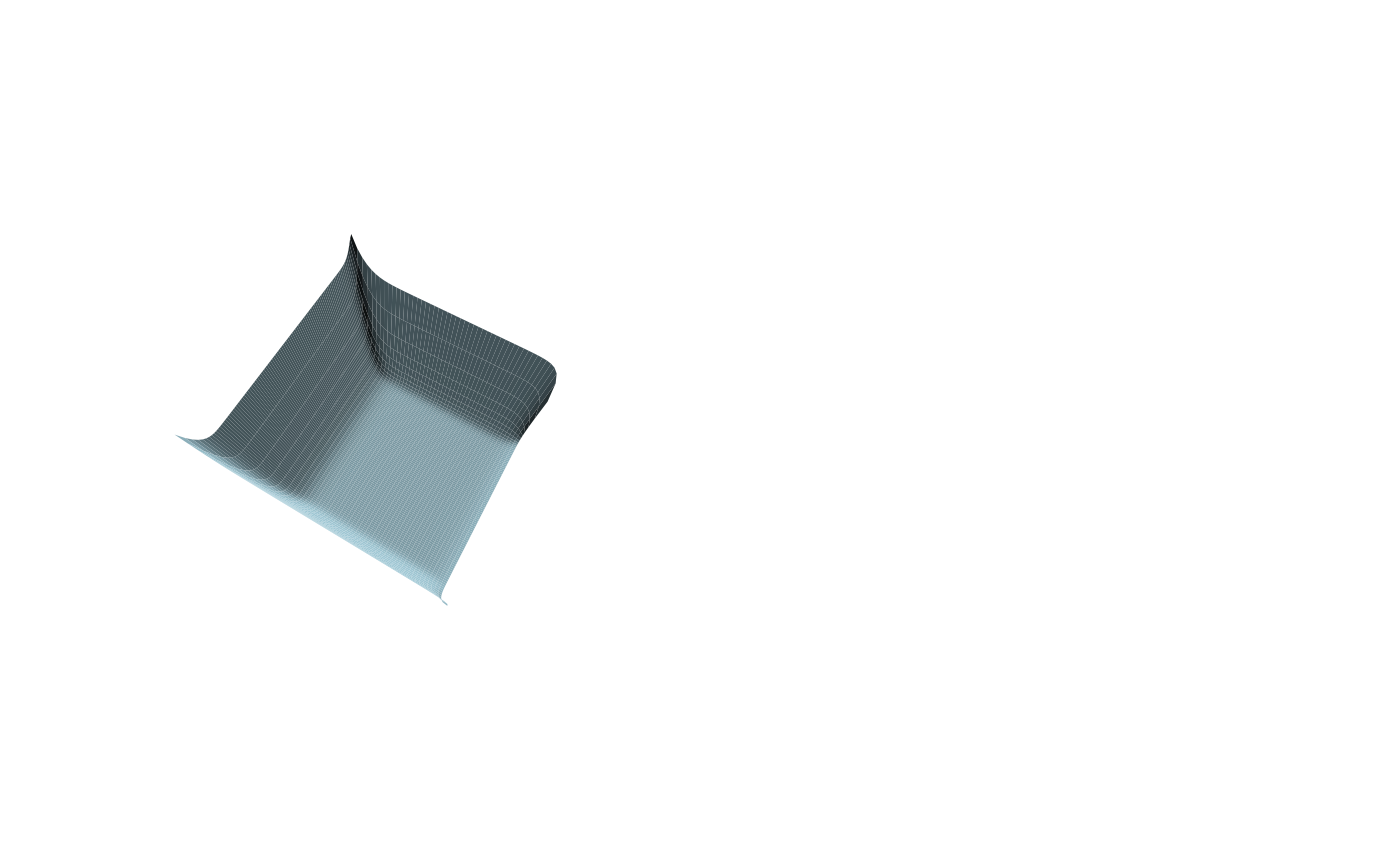
t10 <- matrix (nrow = nx, ncol = ny,
data = subset(ST3, select = "Y", subset = (time == 10)))
persp(t10, theta = 30, border = NA, phi = 70,
col = "lightblue", shade = 0.5, box = FALSE)
# image plot, using deSolve's image function
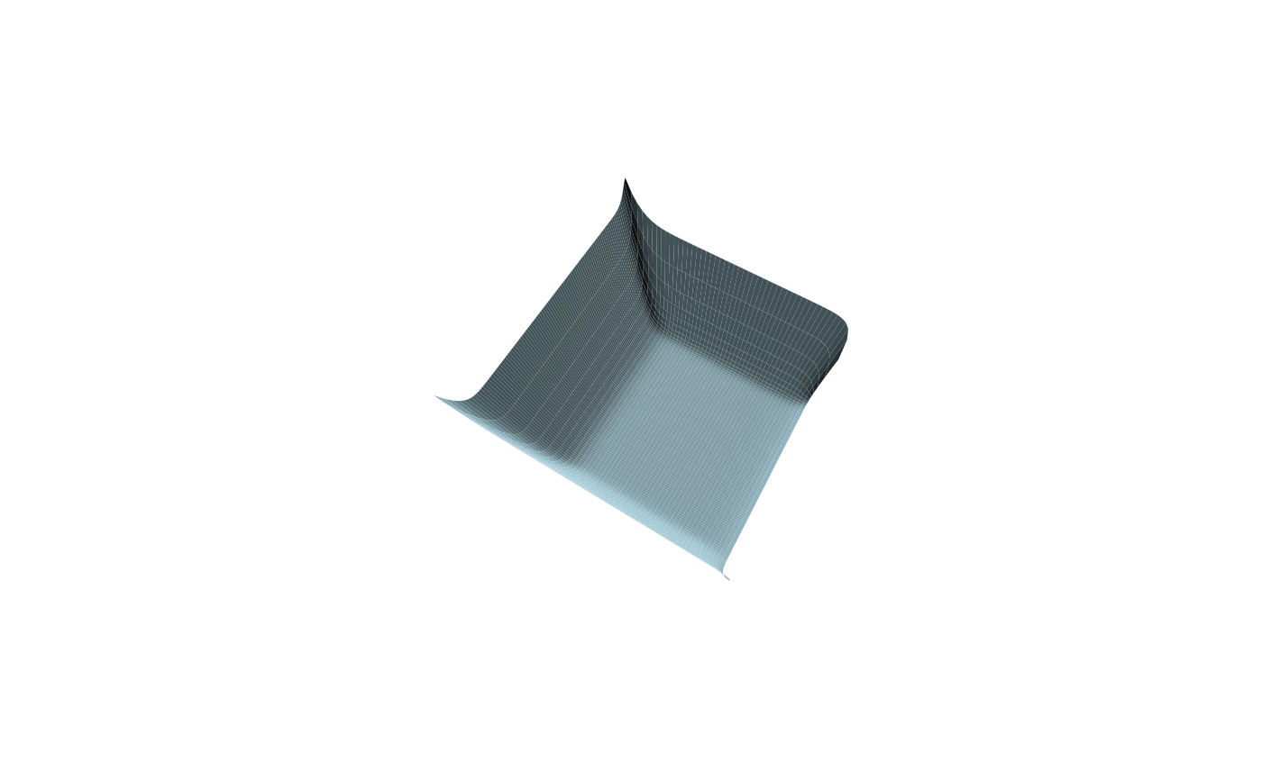
image(ST3, subset = time == 10, method = "persp",
theta = 30, border = NA, phi = 70, main = "",
col = "lightblue", shade = 0.5, box = FALSE)
## =======================================================================
## An example with a cyclic boundary condition.
## Diffusion in 2-D; extra flux on 2 boundaries,
## cyclic boundary in y
## =======================================================================
diffusion2D <- function(t, Y, par) {
y <- matrix(nrow = nx, ncol = ny, data = Y) # vector to 2-D matrix
dY <- -r * y # consumption
BNDx <- rep(1, nx) # boundary concentration
BNDy <- rep(1, ny) # boundary concentration
## diffusion in X-direction; boundaries=imposed concentration
Flux <- -Dx * rbind(y[1,] - BNDy, (y[2:nx,] - y[1:(nx-1),]), BNDy - y[nx,])/dx
dY <- dY - (Flux[2:(nx+1),] - Flux[1:nx,])/dx
## diffusion in Y-direction
Flux <- -Dy * cbind(y[,1] - BNDx, (y[,2:ny]-y[,1:(ny-1)]), BNDx - y[,ny])/dy
dY <- dY - (Flux[,2:(ny+1)] - Flux[,1:ny])/dy
## extra flux on two sides
dY[,1] <- dY[,1] + 10
dY[1,] <- dY[1,] + 10
## and exchange between sides on y-direction
dY[,ny] <- dY[,ny] + (y[,1] - y[,ny]) * 10
return(list(as.vector(dY)))
}
## parameters
dy <- dx <- 1 # grid size
Dy <- Dx <- 1 # diffusion coeff, X- and Y-direction
r <- 0.05 # consumption rate
nx <- 50
ny <- 100
y <- matrix(nrow = nx, ncol = ny, 1)
## model most efficiently solved with lsodes - need to specify lrw
print(system.time(
ST3 <- ode.2D(y, times = 1:100, func = diffusion2D, parms = NULL,
dimens = c(nx, ny), verbose = TRUE, names = "Y",
lrw = 400000, atol = 1e-10, rtol = 1e-10, cyclicBnd = 2)
))
#>
#> --------------------
#> Time settings
#> --------------------
#>
#> Normal computation of output values of y(t) at t = TOUT
#>
#> --------------------
#> Integration settings
#> --------------------
#>
#> Model function an R-function:
#> Jacobian not specified
#>
#>
#> --------------------
#> Integration method
#> --------------------
#>
#> The nonzero elements are according to a 2-D model,
#> the Jacobian will be estimated internally, by differences
#>
#> --------------------
#> lsodes return code
#> --------------------
#>
#> return code (idid) = 2
#> Integration was successful.
#>
#> --------------------
#> INTEGER values
#> --------------------
#>
#> 1 The return code : 2
#> 2 The number of steps taken for the problem so far: 529
#> 3 The number of function evaluations for the problem so far: 664
#> 5 The method order last used (successfully): 5
#> 6 The order of the method to be attempted on the next step: 5
#> 7 If return flag =-4,-5: the largest component in error vector 0
#> 8 The length of the real work array actually required: 376027
#> 9 The length of the integer work array actually required: 29831
#> 14 The number of Jacobian evaluations and LU decompositions so far: 11
#> 17 The number of nonzero elements in the sparse Jacobian: 24800
#>
#> --------------------
#> RSTATE values
#> --------------------
#>
#> 1 The step size in t last used (successfully): 1
#> 2 The step size to be attempted on the next step: 1
#> 3 The current value of the independent variable which the solver has reached: 100.786
#> 4 Tolerance scale factor > 1.0 computed when requesting too much accuracy: 0
#>
#> user system elapsed
#> 0.745 0.002 0.747
# summary of 2-D variable
summary(ST3)
#> Y
#> Min. 2.667149e-02
#> 1st Qu. 2.627932e-01
#> Median 6.615007e-01
#> Mean 1.636228e+00
#> 3rd Qu. 1.887133e+00
#> Max. 1.031178e+01
#> N 5.000000e+05
#> sd 2.216479e+00
# plot output at t = 10
t10 <- matrix (nrow = nx, ncol = ny,
data = subset(ST3, select = "Y", subset = (time == 10)))
persp(t10, theta = 30, border = NA, phi = 70,
col = "lightblue", shade = 0.5, box = FALSE)
# image plot, using deSolve's image function
image(ST3, subset = time == 10, method = "persp",
theta = 30, border = NA, phi = 70, main = "",
col = "lightblue", shade = 0.5, box = FALSE)
 if (FALSE) { # \dontrun{
zlim <- range(ST3[, -1])
for (i in 2:nrow(ST3)) {
y <- matrix(nrow = nx, ncol = ny, data = ST3[i, -1])
filled.contour(y, zlim = zlim, main = i)
}
# same
image(ST3, method = "filled.contour")
} # }
if (FALSE) { # \dontrun{
zlim <- range(ST3[, -1])
for (i in 2:nrow(ST3)) {
y <- matrix(nrow = nx, ncol = ny, data = ST3[i, -1])
filled.contour(y, zlim = zlim, main = i)
}
# same
image(ST3, method = "filled.contour")
} # }