Solver for Differential Algebraic Equations (DAE)
daspk.RdSolves either:
a system of ordinary differential equations (ODE) of the form $$y' = f(t, y, ...)$$ or
a system of differential algebraic equations (DAE) of the form $$F(t,y,y') = 0$$ or
a system of linearly implicit DAES in the form $$M y' = f(t, y)$$
using a combination of backward differentiation formula (BDF) and a direct linear system solution method (dense or banded).
The R function daspk provides an interface to the FORTRAN DAE
solver of the same name, written by Linda R. Petzold, Peter N. Brown,
Alan C. Hindmarsh and Clement W. Ulrich.
The system of DE's is written as an R function (which may, of course,
use .C, .Fortran, .Call, etc., to
call foreign code) or be defined in compiled code that has been
dynamically loaded.
Usage
daspk(y, times, func = NULL, parms, nind = c(length(y), 0, 0),
  dy = NULL, res = NULL, nalg = 0,
  rtol = 1e-6, atol = 1e-6, jacfunc = NULL,
  jacres = NULL, jactype = "fullint", mass = NULL, estini = NULL,
  verbose = FALSE, tcrit = NULL, hmin = 0, hmax = NULL,
  hini = 0, ynames = TRUE, maxord = 5, bandup = NULL,
  banddown = NULL, maxsteps = 5000, dllname = NULL,
  initfunc = dllname, initpar = parms, rpar = NULL,
  ipar = NULL, nout = 0, outnames = NULL,
  forcings=NULL, initforc = NULL, fcontrol=NULL,
  events = NULL, lags = NULL, ...)
Arguments
- y
the initial (state) values for the DE system. If
yhas a name attribute, the names will be used to label the output matrix.- times
time sequence for which output is wanted; the first value of
timesmust be the initial time; if only one step is to be taken; settimes=NULL.- func
to be used if the model is an ODE, or a DAE written in linearly implicit form (M y' = f(t, y)).
funcshould be an R-function that computes the values of the derivatives in the ODE system (the model definition) at time t.funcmust be defined as:func <- function(t, y, parms,...).tis the current time point in the integration,yis the current estimate of the variables in the ODE system. If the initial valuesyhas anamesattribute, the names will be available insidefunc, unlessynamesis FALSE.parmsis a vector or list of parameters....(optional) are any other arguments passed to the function.The return value of
funcshould be a list, whose first element is a vector containing the derivatives ofywith respect totime, and whose next elements are global values that are required at each point intimes. The derivatives should be specified in the same order as the specification of the state variablesy.Note that it is not possible to define
funcas a compiled function in a dynamically loaded shared library. Useresinstead.- parms
vector or list of parameters used in
func,jacfunc, orres- nind
if a DAE system: a three-valued vector with the number of variables of index 1, 2, 3 respectively. The equations must be defined such that the index 1 variables precede the index 2 variables which in turn precede the index 3 variables. The sum of the variables of different index should equal N, the total number of variables. Note that this has been added for consistency with radau. If used, then the variables are weighed differently than in the original daspk code, i.e. index 2 variables are scaled with 1/h, index 3 variables are scaled with 1/h^2. In some cases this allows daspk to solve index 2 or index 3 problems.
- dy
the initial derivatives of the state variables of the DE system. Ignored if an ODE.
- res
if a DAE system: either an R-function that computes the residual function \(F(t,y,y')\) of the DAE system (the model defininition) at time
t, or a character string giving the name of a compiled function in a dynamically loaded shared library.If
resis a user-supplied R-function, it must be defined as:res <- function(t, y, dy, parms, ...).Here
tis the current time point in the integration,yis the current estimate of the variables in the ODE system,dyare the corresponding derivatives. If the initialyordyhave anamesattribute, the names will be available insideres, unlessynamesisFALSE.parmsis a vector of parameters.The return value of
resshould be a list, whose first element is a vector containing the residuals of the DAE system, i.e. \(\delta = F(t,y,y')\), and whose next elements contain output variables that are required at each point intimes.If
resis a string, thendllnamemust give the name of the shared library (without extension) which must be loaded beforedaspk()is called (see package vignette"compiledCode"for more information).- nalg
if a DAE system: the number of algebraic equations (equations not involving derivatives). Algebraic equations should always be the last, i.e. preceeded by the differential equations.
Only used if
estini= 1.- rtol
relative error tolerance, either a scalar or a vector, one value for each y,
- atol
absolute error tolerance, either a scalar or a vector, one value for each y.
- jacfunc
if not
NULL, an R function that computes the Jacobian of the system of differential equations. Only used in case the system is an ODE (\(y' = f(t, y)\)), specified byfunc. The R calling sequence forjacfuncis identical to that offunc.If the Jacobian is a full matrix,
jacfuncshould return a matrix \(\partial\dot{y}/\partial y\), where the ith row contains the derivative of \(dy_i/dt\) with respect to \(y_j\), or a vector containing the matrix elements by columns (the way R and FORTRAN store matrices).If the Jacobian is banded,
jacfuncshould return a matrix containing only the nonzero bands of the Jacobian, rotated row-wise. See first example of lsode.- jacres
jacresand notjacfuncshould be used if the system is specified by the residual function \(F(t, y, y')\), i.e.jacresis used in conjunction withres.If
jacresis an R-function, the calling sequence forjacresis identical to that ofres, but with extra parametercj. Thus it should be called as:jacres = func(t, y, dy, parms, cj, ...). Heretis the current time point in the integration,yis the current estimate of the variables in the ODE system, \(y'\) are the corresponding derivatives andcjis a scalar, which is normally proportional to the inverse of the stepsize. If the initialyordyhave anamesattribute, the names will be available insidejacres, unlessynamesisFALSE.parmsis a vector of parameters (which may have a names attribute).If the Jacobian is a full matrix,
jacresshould return the matrix \(dG/dy + c_j\cdot dG/dy'\), where the \(i\)th row is the sum of the derivatives of \(G_i\) with respect to \(y_j\) and the scaled derivatives of \(G_i\) with respect to \(y'_j\).If the Jacobian is banded,
jacresshould return only the nonzero bands of the Jacobian, rotated rowwise. See details for the calling sequence whenjacresis a string.- jactype
the structure of the Jacobian, one of
"fullint","fullusr","bandusr"or"bandint"- either full or banded and estimated internally or by the user.- mass
the mass matrix. If not
NULL, the problem is a linearly implicit DAE and defined as \(M\, dy/dt = f(t,y)\). The mass-matrix \(M\) should be of dimension \(n*n\) where \(n\) is the number of \(y\)-values.If
mass=NULLthen the model is either an ODE or a DAE, specified withres- estini
only if a DAE system, and if initial values of
yanddyare not consistent (i.e. \(F(t,y,dy) \neq 0\)), settingestini= 1 or 2, will solve for them. Ifestini= 1: dy and the algebraic variables are estimated fromy; in this case, the number of algebraic equations must be given (nalg). Ifestini= 2:ywill be estimated fromdy.- verbose
if TRUE: full output to the screen, e.g. will print the
diagnostiscsof the integration - see details.- tcrit
the FORTRAN routine
daspkovershoots its targets (times points in the vectortimes), and interpolates values for the desired time points. If there is a time beyond which integration should not proceed (perhaps because of a singularity), that should be provided intcrit.- hmin
an optional minimum value of the integration stepsize. In special situations this parameter may speed up computations with the cost of precision. Don't use
hminif you don't know why!- hmax
an optional maximum value of the integration stepsize. If not specified,
hmaxis set to the largest difference intimes, to avoid that the simulation possibly ignores short-term events. If 0, no maximal size is specified.- hini
initial step size to be attempted; if 0, the initial step size is determined by the solver
- ynames
logical, if
FALSE, names of state variables are not passed to functionfunc; this may speed up the simulation especially for large models.- maxord
the maximum order to be allowed. Reduce
maxordto save storage space ( <= 5)- bandup
number of non-zero bands above the diagonal, in case the Jacobian is banded (and
jactypeone of "bandint", "bandusr")- banddown
number of non-zero bands below the diagonal, in case the Jacobian is banded (and
jactypeone of "bandint", "bandusr")- maxsteps
maximal number of steps per output interval taken by the solver; will be recalculated to be at least 500 and a multiple of 500; if
verboseisTRUEthe solver will give a warning if more than 500 steps are taken, but it will continue tillmaxstepssteps. (Note this warning was always given in deSolve versions < 1.10.3).- dllname
a string giving the name of the shared library (without extension) that contains all the compiled function or subroutine definitions referred to in
resandjacres. See package vignette"compiledCode".- initfunc
if not
NULL, the name of the initialisation function (which initialises values of parameters), as provided indllname. See package vignette"compiledCode".- initpar
only when
dllnameis specified and an initialisation functioninitfuncis in the dll: the parameters passed to the initialiser, to initialise the common blocks (FORTRAN) or global variables (C, C++).- rpar
only when
dllnameis specified: a vector with double precision values passed to the dll-functions whose names are specified byresandjacres.- ipar
only when
dllnameis specified: a vector with integer values passed to the dll-functions whose names are specified byresandjacres.- nout
only used if
dllnameis specified and the model is defined in compiled code: the number of output variables calculated in the compiled functionres, present in the shared library. Note: it is not automatically checked whether this is indeed the number of output variables calculated in the dll - you have to perform this check in the code - See package vignette"compiledCode".- outnames
only used if
dllnameis specified andnout> 0: the names of output variables calculated in the compiled functionres, present in the shared library. These names will be used to label the output matrix.- forcings
only used if
dllnameis specified: a list with the forcing function data sets, each present as a two-columned matrix, with (time,value); interpolation outside the interval [min(times), max(times)] is done by taking the value at the closest data extreme.See forcings or package vignette
"compiledCode".- initforc
if not
NULL, the name of the forcing function initialisation function, as provided indllname. It MUST be present ifforcingshas been given a value. See forcings or package vignette"compiledCode".- fcontrol
A list of control parameters for the forcing functions. See forcings or vignette
compiledCode.- events
A matrix or data frame that specifies events, i.e. when the value of a state variable is suddenly changed. See events for more information.
- lags
A list that specifies timelags, i.e. the number of steps that has to be kept. To be used for delay differential equations. See timelags, dede for more information.
- ...
additional arguments passed to
func,jacfunc,resandjacres, allowing this to be a generic function.
Value
A matrix of class deSolve with up to as many rows as elements in
times and as many
columns as elements in y plus the number of "global" values
returned in the next elements of the return from func or
res, plus an additional column (the first) for the time value.
There will be one row for each element in times unless the
FORTRAN routine `daspk' returns with an unrecoverable error. If
y has a names attribute, it will be used to label the columns
of the output value.
References
L. R. Petzold, A Description of DASSL: A Differential/Algebraic System Solver, in Scientific Computing, R. S. Stepleman et al. (Eds.), North-Holland, Amsterdam, 1983, pp. 65-68.
K. E. Brenan, S. L. Campbell, and L. R. Petzold, Numerical Solution of Initial-Value Problems in Differential-Algebraic Equations, Elsevier, New York, 1989.
P. N. Brown and A. C. Hindmarsh, Reduced Storage Matrix Methods in Stiff ODE Systems, J. Applied Mathematics and Computation, 31 (1989), pp. 40-91. doi:10.1016/0096-3003(89)90110-0
P. N. Brown, A. C. Hindmarsh, and L. R. Petzold, Using Krylov Methods in the Solution of Large-Scale Differential-Algebraic Systems, SIAM J. Sci. Comp., 15 (1994), pp. 1467-1488. doi:10.1137/0915088
P. N. Brown, A. C. Hindmarsh, and L. R. Petzold, Consistent Initial Condition Calculation for Differential-Algebraic Systems, LLNL Report UCRL-JC-122175, August 1995; submitted to SIAM J. Sci. Comp.
Netlib: https://netlib.org
Details
The daspk solver uses the backward differentiation formulas of orders
one through five (specified with maxord) to solve either:
an ODE system of the form $$y' = f(t,y,...)$$ or
a DAE system of the form $$y' = M f(t,y,...)$$ or
a DAE system of the form $$F(t,y,y') = 0$$. The index of the DAE should be preferable <= 1.
ODEs are specified using argument func,
DAEs are specified using argument res.
If a DAE system, Values for y and y' (argument dy)
at the initial time must be given as input. Ideally, these values should be consistent,
that is, if t, y, y' are the given initial values, they should
satisfy F(t,y,y') = 0.
However, if consistent values are not
known, in many cases daspk can solve for them: when estini = 1,
y' and algebraic variables (their number specified with nalg)
will be estimated, when estini = 2, y will be estimated.
The form of the Jacobian can be specified by
jactype. This is one of:
- jactype = "fullint":
a full Jacobian, calculated internally by
daspk, the default,- jactype = "fullusr":
a full Jacobian, specified by user function
jacfuncorjacres,- jactype = "bandusr":
a banded Jacobian, specified by user function
jacfuncorjacres; the size of the bands specified bybandupandbanddown,- jactype = "bandint":
a banded Jacobian, calculated by
daspk; the size of the bands specified bybandupandbanddown.
If jactype = "fullusr" or "bandusr" then the user must supply a
subroutine jacfunc.
If jactype = "fullusr" or "bandusr" then the user must supply a
subroutine jacfunc or jacres.
The input parameters rtol, and atol determine the
error control performed by the solver. If the request for
precision exceeds the capabilities of the machine, daspk will return
an error code. See lsoda for details.
When the index of the variables is specified (argument nind),
and higher index variables
are present, then the equations are scaled such that equations corresponding
to index 2 variables are multiplied with 1/h, for index 3 they are multiplied
with 1/h^2, where h is the time step. This is not in the standard DASPK code,
but has been added for consistency with solver radau. Because of this,
daspk can solve certain index 2 or index 3 problems.
res and jacres may be defined in compiled C or FORTRAN code, as
well as in an R-function. See package vignette "compiledCode"
for details. Examples
in FORTRAN are in the dynload subdirectory of the
deSolve package directory.
The diagnostics of the integration can be printed to screen
by calling diagnostics. If verbose = TRUE,
the diagnostics will written to the screen at the end of the integration.
See vignette("deSolve") for an explanation of each element in the vectors containing the diagnostic properties and how to directly access them.
Models may be defined in compiled C or FORTRAN code, as well as
in an R-function. See package vignette "compiledCode" for details.
More information about models defined in compiled code is in the package vignette ("compiledCode"); information about linking forcing functions to compiled code is in forcings.
Examples in both C and FORTRAN are in the dynload subdirectory
of the deSolve package directory.
See also
radaufor integrating DAEs up to index 3,rk,lsoda,lsode,lsodes,lsodar,vode, for other solvers of the Livermore family,odefor a general interface to most of the ODE solvers,ode.bandfor solving models with a banded Jacobian,ode.1Dfor integrating 1-D models,ode.2Dfor integrating 2-D models,ode.3Dfor integrating 3-D models,
diagnostics to print diagnostic messages.
Note
In this version, the Krylov method is not (yet) supported.
From deSolve version 1.10.4 and above, the following changes were made
the argument list to
daspknow also includesnind, the index of each variable. This is used to scale the variables, such thatdaspkin R can also solve certain index 2 or index 3 problems, which the original Fortran version may not be able to solve.the default of
atolwas changed from 1e-8 to 1e-6, to be consistent with the other solvers.the multiple warnings from daspk when the number of steps exceed 500 were toggled off unless
verboseisTRUE
Examples
## =======================================================================
## Coupled chemical reactions including an equilibrium
## modeled as (1) an ODE and (2) as a DAE
##
## The model describes three chemical species A,B,D:
## subjected to equilibrium reaction D <- > A + B
## D is produced at a constant rate, prod
## B is consumed at 1s-t order rate, r
## Chemical problem formulation 1: ODE
## =======================================================================
## Dissociation constant
K <- 1
## parameters
pars <- c(
ka = 1e6, # forward rate
r = 1,
prod = 0.1)
Fun_ODE <- function (t, y, pars)
{
with (as.list(c(y, pars)), {
ra <- ka*D # forward rate
rb <- ka/K *A*B # backward rate
## rates of changes
dD <- -ra + rb + prod
dA <- ra - rb
dB <- ra - rb - r*B
return(list(dy = c(dA, dB, dD),
CONC = A+B+D))
})
}
## =======================================================================
## Chemical problem formulation 2: DAE
## 1. get rid of the fast reactions ra and rb by taking
## linear combinations : dD+dA = prod (res1) and
## dB-dA = -r*B (res2)
## 2. In addition, the equilibrium condition (eq) reads:
## as ra = rb : ka*D = ka/K*A*B = > K*D = A*B
## =======================================================================
Res_DAE <- function (t, y, yprime, pars)
{
with (as.list(c(y, yprime, pars)), {
## residuals of lumped rates of changes
res1 <- -dD - dA + prod
res2 <- -dB + dA - r*B
## and the equilibrium equation
eq <- K*D - A*B
return(list(c(res1, res2, eq),
CONC = A+B+D))
})
}
## =======================================================================
## Chemical problem formulation 3: Mass * Func
## Based on the DAE formulation
## =======================================================================
Mass_FUN <- function (t, y, pars) {
with (as.list(c(y, pars)), {
## as above, but without the
f1 <- prod
f2 <- - r*B
## and the equilibrium equation
f3 <- K*D - A*B
return(list(c(f1, f2, f3),
CONC = A+B+D))
})
}
Mass <- matrix(nrow = 3, ncol = 3, byrow = TRUE,
data=c(1, 0, 1, # dA + 0 + dB
-1, 1, 0, # -dA + dB +0
0, 0, 0)) # algebraic
times <- seq(0, 100, by = 2)
## Initial conc; D is in equilibrium with A,B
y <- c(A = 2, B = 3, D = 2*3/K)
## ODE model solved with daspk
ODE <- daspk(y = y, times = times, func = Fun_ODE,
parms = pars, atol = 1e-10, rtol = 1e-10)
## Initial rate of change
dy <- c(dA = 0, dB = 0, dD = 0)
## DAE model solved with daspk
DAE <- daspk(y = y, dy = dy, times = times,
res = Res_DAE, parms = pars, atol = 1e-10, rtol = 1e-10)
MASS<- daspk(y=y, times=times, func = Mass_FUN, parms = pars, mass = Mass)
## ================
## plotting output
## ================
plot(ODE, DAE, xlab = "time", ylab = "conc", type = c("l", "p"),
pch = c(NA, 1))
legend("bottomright", lty = c(1, NA), pch = c(NA, 1),
col = c("black", "red"), legend = c("ODE", "DAE"))
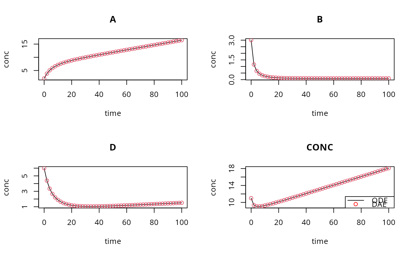 # difference between both implementations:
max(abs(ODE-DAE))
#> [1] 2.731114e-07
## =======================================================================
## same DAE model, now with the Jacobian
## =======================================================================
jacres_DAE <- function (t, y, yprime, pars, cj)
{
with (as.list(c(y, yprime, pars)), {
## res1 = -dD - dA + prod
PD[1,1] <- -1*cj # d(res1)/d(A)-cj*d(res1)/d(dA)
PD[1,2] <- 0 # d(res1)/d(B)-cj*d(res1)/d(dB)
PD[1,3] <- -1*cj # d(res1)/d(D)-cj*d(res1)/d(dD)
## res2 = -dB + dA - r*B
PD[2,1] <- 1*cj
PD[2,2] <- -r -1*cj
PD[2,3] <- 0
## eq = K*D - A*B
PD[3,1] <- -B
PD[3,2] <- -A
PD[3,3] <- K
return(PD)
})
}
PD <- matrix(ncol = 3, nrow = 3, 0)
DAE2 <- daspk(y = y, dy = dy, times = times,
res = Res_DAE, jacres = jacres_DAE, jactype = "fullusr",
parms = pars, atol = 1e-10, rtol = 1e-10)
max(abs(DAE-DAE2))
#> [1] 1.725007e-09
## See \dynload subdirectory for a FORTRAN implementation of this model
## =======================================================================
## The chemical model as a DLL, with production a forcing function
## =======================================================================
times <- seq(0, 100, by = 2)
pars <- c(K = 1, ka = 1e6, r = 1)
## Initial conc; D is in equilibrium with A,B
y <- c(A = 2, B = 3, D = as.double(2*3/pars["K"]))
## Initial rate of change
dy <- c(dA = 0, dB = 0, dD = 0)
# production increases with time
prod <- matrix(ncol = 2,
data = c(seq(0, 100, by = 10), 0.1*(1+runif(11)*1)))
ODE_dll <- daspk(y = y, dy = dy, times = times, res = "chemres",
dllname = "deSolve", initfunc = "initparms",
initforc = "initforcs", parms = pars, forcings = prod,
atol = 1e-10, rtol = 1e-10, nout = 2,
outnames = c("CONC","Prod"))
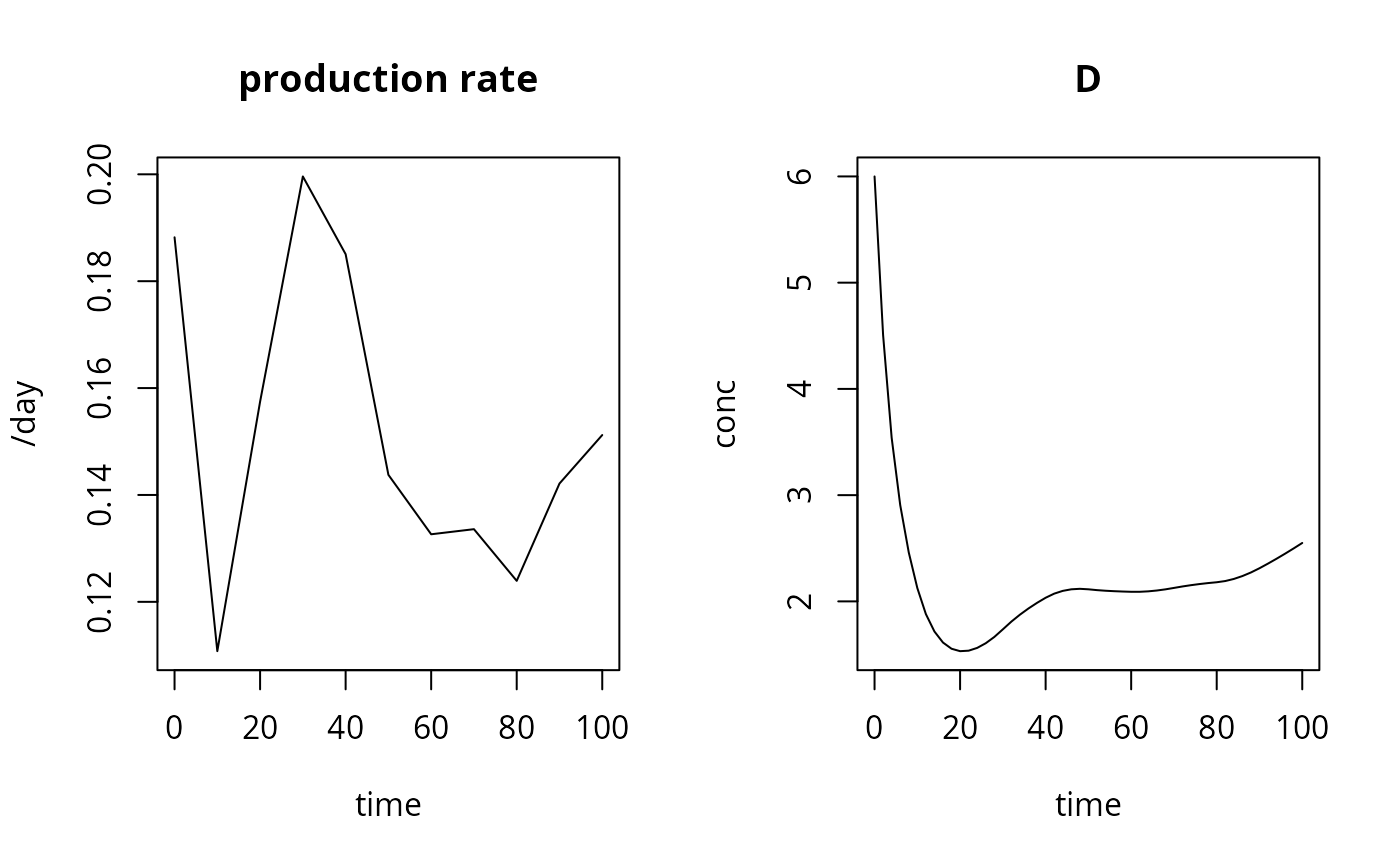
plot(ODE_dll, which = c("Prod", "D"), xlab = "time",
ylab = c("/day", "conc"), main = c("production rate","D"))
# difference between both implementations:
max(abs(ODE-DAE))
#> [1] 2.731114e-07
## =======================================================================
## same DAE model, now with the Jacobian
## =======================================================================
jacres_DAE <- function (t, y, yprime, pars, cj)
{
with (as.list(c(y, yprime, pars)), {
## res1 = -dD - dA + prod
PD[1,1] <- -1*cj # d(res1)/d(A)-cj*d(res1)/d(dA)
PD[1,2] <- 0 # d(res1)/d(B)-cj*d(res1)/d(dB)
PD[1,3] <- -1*cj # d(res1)/d(D)-cj*d(res1)/d(dD)
## res2 = -dB + dA - r*B
PD[2,1] <- 1*cj
PD[2,2] <- -r -1*cj
PD[2,3] <- 0
## eq = K*D - A*B
PD[3,1] <- -B
PD[3,2] <- -A
PD[3,3] <- K
return(PD)
})
}
PD <- matrix(ncol = 3, nrow = 3, 0)
DAE2 <- daspk(y = y, dy = dy, times = times,
res = Res_DAE, jacres = jacres_DAE, jactype = "fullusr",
parms = pars, atol = 1e-10, rtol = 1e-10)
max(abs(DAE-DAE2))
#> [1] 1.725007e-09
## See \dynload subdirectory for a FORTRAN implementation of this model
## =======================================================================
## The chemical model as a DLL, with production a forcing function
## =======================================================================
times <- seq(0, 100, by = 2)
pars <- c(K = 1, ka = 1e6, r = 1)
## Initial conc; D is in equilibrium with A,B
y <- c(A = 2, B = 3, D = as.double(2*3/pars["K"]))
## Initial rate of change
dy <- c(dA = 0, dB = 0, dD = 0)
# production increases with time
prod <- matrix(ncol = 2,
data = c(seq(0, 100, by = 10), 0.1*(1+runif(11)*1)))
ODE_dll <- daspk(y = y, dy = dy, times = times, res = "chemres",
dllname = "deSolve", initfunc = "initparms",
initforc = "initforcs", parms = pars, forcings = prod,
atol = 1e-10, rtol = 1e-10, nout = 2,
outnames = c("CONC","Prod"))
plot(ODE_dll, which = c("Prod", "D"), xlab = "time",
ylab = c("/day", "conc"), main = c("production rate","D"))