Implicit Runge-Kutta RADAU IIA

Solves the initial value problem for stiff or nonstiff systems of ordinary differential equations (ODE) in the form: $$dy/dt = f(t,y)$$ or linearly implicit differential algebraic equations in the form: $$M dy/dt = f(t,y)$$.

The R function radau provides an interface to the Fortran solver RADAU5, written by Ernst Hairer and G. Wanner, which implements the 3-stage RADAU IIA method. It implements the implicit Runge-Kutta method of order 5 with step size control and continuous output. The system of ODEs or DAEs is written as an R function or can be defined in compiled code that has been dynamically loaded.

Usage

radau(y, times, func, parms, nind = c(length(y), 0, 0), 
  rtol = 1e-6, atol = 1e-6, jacfunc = NULL, jactype = "fullint", 
  mass = NULL, massup = NULL, massdown = NULL, rootfunc = NULL,
  verbose = FALSE, nroot = 0, hmax = NULL, hini = 0, ynames = TRUE,
  bandup = NULL, banddown = NULL, maxsteps = 5000, 
  dllname = NULL, initfunc = dllname, initpar = parms, 
  rpar = NULL, ipar = NULL, nout = 0, outnames = NULL, 
  forcings = NULL, initforc = NULL, fcontrol = NULL,
  events=NULL, lags = NULL, ...)

Arguments

y

the initial (state) values for the ODE system. If y has a name attribute, the names will be used to label the output matrix.

times

time sequence for which output is wanted; the first value of times must be the initial time; if only one step is to be taken; set times = NULL.

func

either an R-function that computes the values of the derivatives in the ODE system (the model definition) at time t, or the right-hand side of the equation $$M dy/dt = f(t,y)$$ if a DAE. (if mass is supplied then the problem is assumed a DAE).

func can also be a character string giving the name of a compiled function in a dynamically loaded shared library.

If func is an R-function, it must be defined as:

func <- function(t, y, parms,...).

t is the current time point in the integration, y is the current estimate of the variables in the ODE system. If the initial values y has a names attribute, the names will be available inside func. parms is a vector or list of parameters; ... (optional) are any other arguments passed to the function.

The return value of func should be a list, whose first element is a vector containing the derivatives of y with respect to time, and whose next elements are global values that are required at each point in times. The derivatives must be specified in the same order as the state variables y.

If func is a string, then dllname must give the name of the shared library (without extension) which must be loaded before radau() is called. See deSolve package vignette "compiledCode" for more details.

parms

vector or list of parameters used in func or jacfunc.

nind

if a DAE system: a three-valued vector with the number of variables of index 1, 2, 3 respectively. The equations must be defined such that the index 1 variables precede the index 2 variables which in turn precede the index 3 variables. The sum of the variables of different index should equal N, the total number of variables. This has implications on the scaling of the variables, i.e. index 2 variables are scaled by 1/h, index 3 variables are scaled by 1/h^2.

rtol

relative error tolerance, either a scalar or an array as long as y. See details.

atol

absolute error tolerance, either a scalar or an array as long as y. See details.

jacfunc

if not NULL, an R function that computes the Jacobian of the system of differential equations $\partial\dot{y}_i/\partial y_j$, or a string giving the name of a function or subroutine in dllname that computes the Jacobian (see vignette "compiledCode" from package deSolve, for more about this option).

In some circumstances, supplying jacfunc can speed up the computations, if the system is stiff. The R calling sequence for jacfunc is identical to that of func.

If the Jacobian is a full matrix, jacfunc should return a matrix $\partial\dot{y}/\partial y$, where the ith row contains the derivative of $dy_i/dt$ with respect to $y_j$, or a vector containing the matrix elements by columns (the way R and FORTRAN store matrices).
If the Jacobian is banded, jacfunc should return a matrix containing only the nonzero bands of the Jacobian, rotated row-wise. See example.

jactype

the structure of the Jacobian, one of "fullint", "fullusr", "bandusr" or "bandint" - either full or banded and estimated internally or by user.

mass

the mass matrix. If not NULL, the problem is a linearly implicit DAE and defined as $M\, dy/dt = f(t,y)$. If the mass-matrix $M$ is full, it should be of dimension $n^2$ where $n$ is the number of $y$-values; if banded the number of rows should be less than $n$, and the mass-matrix is stored diagonal-wise with element $(i, j)$ stored in mass(i - j + mumas + 1, j).

If mass = NULL then the model is an ODE (default)

massup

number of non-zero bands above the diagonal of the mass matrix, in case it is banded.

massdown

number of non-zero bands below the diagonal of the mass matrix, in case it is banded.

rootfunc

if not NULL, an R function that computes the function whose root has to be estimated or a string giving the name of a function or subroutine in dllname that computes the root function. The R calling sequence for rootfunc is identical to that of func. rootfunc should return a vector with the function values whose root is sought.

verbose

if TRUE: full output to the screen, e.g. will print the diagnostiscs of the integration - see details.

nroot

only used if dllname is specified: the number of constraint functions whose roots are desired during the integration; if rootfunc is an R-function, the solver estimates the number of roots.

hmax

an optional maximum value of the integration stepsize. If not specified, hmax is set to the largest difference in times, to avoid that the simulation possibly ignores short-term events. If 0, no maximal size is specified.

hini

initial step size to be attempted; if 0, the initial step size is set equal to 1e-6. Usually 1e-3 to 1e-5 is good for stiff equations

ynames

logical, if FALSE names of state variables are not passed to function func; this may speed up the simulation especially for multi-D models.

bandup

number of non-zero bands above the diagonal, in case the Jacobian is banded.

banddown

number of non-zero bands below the diagonal, in case the Jacobian is banded.

maxsteps

average maximal number of steps per output interval taken by the solver. This argument is defined such as to ensure compatibility with the Livermore-solvers. RADAU only accepts the maximal number of steps for the entire integration, and this is calculated as length(times) * maxsteps.

dllname

a string giving the name of the shared library (without extension) that contains all the compiled function or subroutine definitions refered to in func and jacfunc. See vignette "compiledCode" from package deSolve.

initfunc

if not NULL, the name of the initialisation function (which initialises values of parameters), as provided in dllname. See vignette "compiledCode" from package deSolve.

initpar

only when dllname is specified and an initialisation function initfunc is in the dll: the parameters passed to the initialiser, to initialise the common blocks (FORTRAN) or global variables (C, C++).

rpar

only when dllname is specified: a vector with double precision values passed to the dll-functions whose names are specified by func and jacfunc.

ipar

only when dllname is specified: a vector with integer values passed to the dll-functions whose names are specified by func and jacfunc.

nout

only used if dllname is specified and the model is defined in compiled code: the number of output variables calculated in the compiled function func, present in the shared library. Note: it is not automatically checked whether this is indeed the number of output variables calculed in the DLL - you have to perform this check in the code - See vignette "compiledCode" from package deSolve.

outnames

only used if dllname is specified and nout > 0: the names of output variables calculated in the compiled function func, present in the shared library. These names will be used to label the output matrix.

forcings

only used if dllname is specified: a list with the forcing function data sets, each present as a two-columned matrix, with (time, value); interpolation outside the interval [min(times), max(times)] is done by taking the value at the closest data extreme.

See forcings or package vignette "compiledCode".

initforc

if not NULL, the name of the forcing function initialisation function, as provided in dllname. It MUST be present if forcings has been given a value. See forcings or package vignette "compiledCode".

fcontrol

A list of control parameters for the forcing functions. See forcings or vignette compiledCode.

events

A matrix or data frame that specifies events, i.e. when the value of a state variable is suddenly changed. See events for more information.

lags

A list that specifies timelags, i.e. the number of steps that has to be kept. To be used for delay differential equations. See timelags, dede for more information.

...

additional arguments passed to func and jacfunc allowing this to be a generic function.

Value

A matrix of class deSolve with up to as many rows as elements in times and as many columns as elements in y plus the number of "global" values returned in the next elements of the return from func, plus and additional column for the time value. There will be a row for each element in times unless the FORTRAN routine returns with an unrecoverable error. If y has a names attribute, it will be used to label the columns of the output value.

Author

Karline Soetaert

References

E. Hairer and G. Wanner, 1996. Solving Ordinary Differential Equations II. Stiff and Differential-algebraic problems. Springer series in computational mathematics 14, Springer-Verlag, second edition.

Details

The work is done by the FORTRAN subroutine RADAU5, whose documentation should be consulted for details. The implementation is based on the Fortran 77 version from January 18, 2002.

There are four standard choices for the Jacobian which can be specified with jactype.

The options for jactype are

jactype = "fullint": a full Jacobian, calculated internally by the solver.
jactype = "fullusr": a full Jacobian, specified by user function jacfunc.
jactype = "bandusr": a banded Jacobian, specified by user function jacfunc; the size of the bands specified by bandup and banddown.
jactype = "bandint": a banded Jacobian, calculated by radau; the size of the bands specified by bandup and banddown.

Inspection of the example below shows how to specify both a banded and full Jacobian.

The input parameters rtol, and atol determine the error control performed by the solver, which roughly keeps the local error of $y(i)$ below $rtol(i)*abs(y(i))+atol(i)$.

The diagnostics of the integration can be printed to screen by calling diagnostics. If verbose = TRUE, the diagnostics will be written to the screen at the end of the integration.

See vignette("deSolve") from the deSolve package for an explanation of each element in the vectors containing the diagnostic properties and how to directly access them.

Models may be defined in compiled C or FORTRAN code, as well as in an R-function. See package vignette "compiledCode" from package deSolve for details.

Information about linking forcing functions to compiled code is in forcings (from package deSolve).

radau can find the root of at least one of a set of constraint functions rootfunc of the independent and dependent variables. It then returns the solution at the root if that occurs sooner than the specified stop condition, and otherwise returns the solution according the specified stop condition.

Caution: Because of numerical errors in the function rootfun due to roundoff and integration error, radau may return false roots, or return the same root at two or more nearly equal values of time.

Examples

## =======================================================================
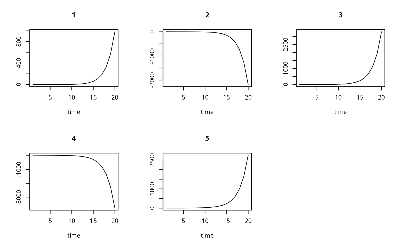
## Example 1: ODE
##   Various ways to solve the same model.
## =======================================================================

## the model, 5 state variables
f1 <- function  (t, y, parms) {
  ydot <- vector(len = 5)

  ydot[1] <-  0.1*y[1] -0.2*y[2]
  ydot[2] <- -0.3*y[1] +0.1*y[2] -0.2*y[3]
  ydot[3] <-           -0.3*y[2] +0.1*y[3] -0.2*y[4]
  ydot[4] <-                     -0.3*y[3] +0.1*y[4] -0.2*y[5]
  ydot[5] <-                               -0.3*y[4] +0.1*y[5]

  return(list(ydot))
}

## the Jacobian, written as a full matrix
fulljac <- function  (t, y, parms) {
  jac <- matrix(nrow = 5, ncol = 5, byrow = TRUE,
                data = c(0.1, -0.2,  0  ,  0  ,  0  ,
                        -0.3,  0.1, -0.2,  0  ,  0  ,
                         0  , -0.3,  0.1, -0.2,  0  ,
                         0  ,  0  , -0.3,  0.1, -0.2,
                         0  ,  0  ,  0  , -0.3,  0.1))
  return(jac)
}

## the Jacobian, written in banded form
bandjac <- function  (t, y, parms) {
  jac <- matrix(nrow = 3, ncol = 5, byrow = TRUE,
                data = c( 0  , -0.2, -0.2, -0.2, -0.2,
                          0.1,  0.1,  0.1,  0.1,  0.1,
                         -0.3, -0.3, -0.3, -0.3,    0))
  return(jac)
}

## initial conditions and output times
yini  <- 1:5
times <- 1:20

## default: stiff method, internally generated, full Jacobian
out   <- radau(yini, times, f1, parms = 0)
plot(out)

## stiff method, user-generated full Jacobian
out2  <- radau(yini, times, f1, parms = 0, jactype = "fullusr",
               jacfunc = fulljac)

## stiff method, internally-generated banded Jacobian
## one nonzero band above (up) and below(down) the diagonal
out3  <- radau(yini, times, f1, parms = 0, jactype = "bandint",
               bandup = 1, banddown = 1)

## stiff method, user-generated banded Jacobian
out4  <- radau(yini, times, f1, parms = 0, jactype = "bandusr",
               jacfunc = bandjac, bandup = 1, banddown = 1)


## =======================================================================
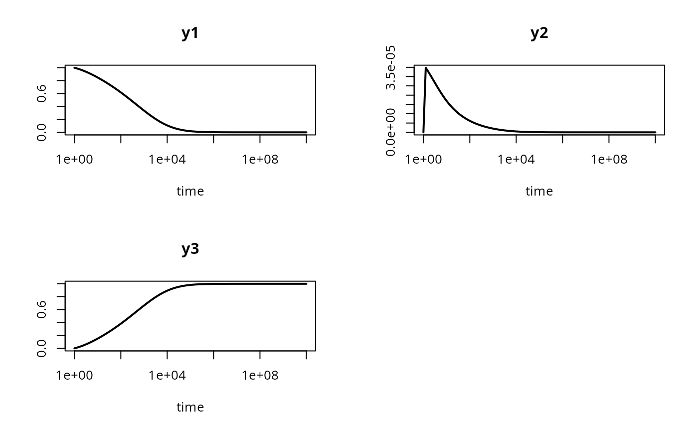
## Example 2: ODE
##   stiff problem from chemical kinetics
## =======================================================================
Chemistry <- function (t, y, p) {
  dy1 <- -.04*y[1] + 1.e4*y[2]*y[3]
  dy2 <- .04*y[1] - 1.e4*y[2]*y[3] - 3.e7*y[2]^2
  dy3 <- 3.e7*y[2]^2
  list(c(dy1, dy2, dy3))
}

times <- 10^(seq(0, 10, by = 0.1))
yini <- c(y1 = 1.0, y2 = 0, y3 = 0)

out <- radau(func = Chemistry, times = times, y = yini, parms = NULL)
plot(out, log = "x", type = "l", lwd = 2)


## =============================================================================
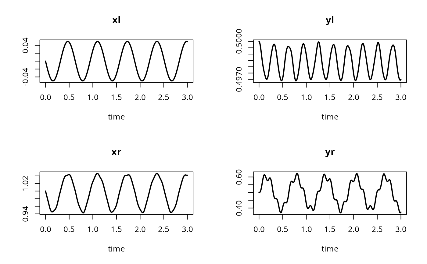
## Example 3: DAE
## Car axis problem, index 3 DAE, 8 differential, 2 algebraic equations
## from
## F. Mazzia and C. Magherini. Test Set for Initial Value Problem Solvers,
## release 2.4. Department
## of Mathematics, University of Bari and INdAM, Research Unit of Bari,
## February 2008.
## Available from https://archimede.uniba.it/~testset/
## =============================================================================

## Problem is written as M*y' = f(t,y,p).
## caraxisfun implements the right-hand side:

caraxisfun <- function(t, y, parms) {
  with(as.list(y), {
  
    yb <- r * sin(w * t)
    xb <- sqrt(L * L - yb * yb)
    Ll <- sqrt(xl^2 + yl^2)
    Lr <- sqrt((xr - xb)^2 + (yr - yb)^2)
        
    dxl <- ul; dyl <- vl; dxr <- ur; dyr <- vr
        
    dul  <- (L0-Ll) * xl/Ll      + 2 * lam2 * (xl-xr) + lam1*xb
    dvl  <- (L0-Ll) * yl/Ll      + 2 * lam2 * (yl-yr) + lam1*yb - k * g
               
    dur  <- (L0-Lr) * (xr-xb)/Lr - 2 * lam2 * (xl-xr)
    dvr  <- (L0-Lr) * (yr-yb)/Lr - 2 * lam2 * (yl-yr) - k * g
        
    c1   <- xb * xl + yb * yl
    c2   <- (xl - xr)^2 + (yl - yr)^2 - L * L
        
    list(c(dxl, dyl, dxr, dyr, dul, dvl, dur, dvr, c1, c2))
  })
}

eps <- 0.01; M <- 10; k <- M * eps^2/2; 
L <- 1; L0 <- 0.5; r <- 0.1; w <- 10; g <- 1

yini <- c(xl = 0, yl = L0, xr = L, yr = L0,
          ul = -L0/L, vl = 0,
          ur = -L0/L, vr = 0,
          lam1 = 0, lam2 = 0)

# the mass matrix
Mass      <- diag(nrow = 10, 1)
Mass[5,5] <- Mass[6,6] <- Mass[7,7] <- Mass[8,8] <- M * eps * eps/2
Mass[9,9] <- Mass[10,10] <- 0
Mass
#>       [,1] [,2] [,3] [,4]  [,5]  [,6]  [,7]  [,8] [,9] [,10]
#>  [1,]    1    0    0    0 0e+00 0e+00 0e+00 0e+00    0     0
#>  [2,]    0    1    0    0 0e+00 0e+00 0e+00 0e+00    0     0
#>  [3,]    0    0    1    0 0e+00 0e+00 0e+00 0e+00    0     0
#>  [4,]    0    0    0    1 0e+00 0e+00 0e+00 0e+00    0     0
#>  [5,]    0    0    0    0 5e-04 0e+00 0e+00 0e+00    0     0
#>  [6,]    0    0    0    0 0e+00 5e-04 0e+00 0e+00    0     0
#>  [7,]    0    0    0    0 0e+00 0e+00 5e-04 0e+00    0     0
#>  [8,]    0    0    0    0 0e+00 0e+00 0e+00 5e-04    0     0
#>  [9,]    0    0    0    0 0e+00 0e+00 0e+00 0e+00    0     0
#> [10,]    0    0    0    0 0e+00 0e+00 0e+00 0e+00    0     0

# index of the variables: 4 of index 1, 4 of index 2, 2 of index 3
index <- c(4, 4, 2)

times <- seq(0, 3, by = 0.01)
out <- radau(y = yini, mass = Mass, times = times, func = caraxisfun,
        parms = NULL, nind = index)

plot(out, which = 1:4, type = "l", lwd = 2)