Explicit One-Step Solvers for Ordinary Differential Equations (ODE)
rk.RdSolving initial value problems for non-stiff systems of first-order ordinary differential equations (ODEs).
The R function rk is a top-level function that provides
interfaces to a collection of common explicit one-step solvers of the
Runge-Kutta family with fixed or variable time steps.
The system of ODE's is written as an R function (which may, of
course, use .C, .Fortran,
.Call, etc., to call foreign code) or be defined in
compiled code that has been dynamically loaded. A vector of
parameters is passed to the ODEs, so the solver may be used as part of
a modeling package for ODEs, or for parameter estimation using any
appropriate modeling tool for non-linear models in R such as
optim, nls, nlm or
nlme
Usage
rk(y, times, func, parms, rtol = 1e-6, atol = 1e-6,
  verbose = FALSE, tcrit = NULL, hmin = 0, hmax = NULL,
  hini = hmax, ynames = TRUE, method = rkMethod("rk45dp7", ... ),
  maxsteps = 5000, dllname = NULL, initfunc = dllname,
  initpar = parms, rpar = NULL, ipar = NULL,
  nout = 0, outnames = NULL, forcings = NULL,
  initforc = NULL, fcontrol = NULL, events = NULL, ...)
Arguments
- y
the initial (state) values for the ODE system. If
yhas a name attribute, the names will be used to label the output matrix.- times
times at which explicit estimates for
yare desired. The first value intimesmust be the initial time.- func
either an R-function that computes the values of the derivatives in the ODE system (the model definition) at time t, or a character string giving the name of a compiled function in a dynamically loaded shared library.
If
funcis an R-function, it must be defined as:func <- function(t, y, parms,...).tis the current time point in the integration,yis the current estimate of the variables in the ODE system. If the initial valuesyhas anamesattribute, the names will be available insidefunc.parmsis a vector or list of parameters; ... (optional) are any other arguments passed to the function.The return value of
funcshould be a list, whose first element is a vector containing the derivatives ofywith respect totime, and whose next elements are global values that are required at each point intimes. The derivatives must be specified in the same order as the state variablesy.If
funcis a string, thendllnamemust give the name of the shared library (without extension) which must be loaded beforerkis called. See package vignette"compiledCode"for more details.- parms
vector or list of parameters used in
func.- rtol
relative error tolerance, either a scalar or an array as long as
y. Only applicable to methods with variable time step, see details.- atol
absolute error tolerance, either a scalar or an array as long as
y. Only applicable to methods with variable time step, see details.- tcrit
if not
NULL, thenrkcannot integrate pasttcrit. This parameter is for compatibility with other solvers.- verbose
a logical value that, when TRUE, triggers more verbose output from the ODE solver.
- hmin
an optional minimum value of the integration stepsize. In special situations this parameter may speed up computations with the cost of precision. Don't use
hminif you don't know why!- hmax
an optional maximum value of the integration stepsize. If not specified,
hmaxis set to the maximum ofhiniand the largest difference intimes, to avoid that the simulation possibly ignores short-term events. If 0, no maximal size is specified. Note thathminandhmaxare ignored by fixed step methods like"rk4"or"euler".- hini
initial step size to be attempted; if 0, the initial step size is determined automatically by solvers with flexible time step. For fixed step methods, setting
hini = 0forces internal time steps identically to external time steps provided bytimes. Similarly, internal time steps of non-interpolating solvers cannot be bigger than external time steps specified intimes.- ynames
if
FALSE: names of state variables are not passed to functionfunc; this may speed up the simulation especially for large models.- method
the integrator to use. This can either be a string constant naming one of the pre-defined methods or a call to function
rkMethodspecifying a user-defined method. The most common methods are the fixed-step methods"euler", second and fourth-order Runge Kutta ("rk2","rk4"), or the variable step methods Bogacki-Shampine"rk23bs", Runge-Kutta-Fehlberg"rk34f", the fifth-order Cash-Karp method"rk45ck"or the fifth-order Dormand-Prince method with seven stages"rk45dp7". As a suggestion, one may use"rk23bs"(alias"ode23") for simple problems and"rk45dp7"(alias"ode45") for rough problems.- maxsteps
average maximal number of steps per output interval taken by the solver. This argument is defined such as to ensure compatibility with the Livermore-solvers.
rkonly accepts the maximal number of steps for the entire integration. It is calculated asmax(length(times) * maxsteps, max(diff(times)/hini + 1).- dllname
a string giving the name of the shared library (without extension) that contains all the compiled function or subroutine definitions refered to in
funcandjacfunc. See package vignette"compiledCode".- initfunc
if not
NULL, the name of the initialisation function (which initialises values of parameters), as provided indllname. See package vignette"compiledCode".- initpar
only when
dllnameis specified and an initialisation functioninitfuncis in the dll: the parameters passed to the initialiser, to initialise the common blocks (FORTRAN) or global variables (C, C++).- rpar
only when
dllnameis specified: a vector with double precision values passed to the dll-functions whose names are specified byfuncandjacfunc.- ipar
only when
dllnameis specified: a vector with integer values passed to the dll-functions whose names are specified byfuncandjacfunc.- nout
only used if
dllnameis specified and the model is defined in compiled code: the number of output variables calculated in the compiled functionfunc, present in the shared library. Note: it is not automatically checked whether this is indeed the number of output variables calculated in the dll - you have to perform this check in the code. See package vignette"compiledCode".- outnames
only used if
dllnameis specified andnout> 0: the names of output variables calculated in the compiled functionfunc, present in the shared library.- forcings
only used if
dllnameis specified: a list with the forcing function data sets, each present as a two-columned matrix, with (time,value); interpolation outside the interval [min(times), max(times)] is done by taking the value at the closest data extreme.See forcings or package vignette
"compiledCode".- initforc
if not
NULL, the name of the forcing function initialisation function, as provided indllname. It MUST be present ifforcingshas been given a value. See forcings or package vignette"compiledCode".- fcontrol
A list of control parameters for the forcing functions. See forcings or vignette
compiledCode.- events
A matrix or data frame that specifies events, i.e. when the value of a state variable is suddenly changed. See events for more information. Not also that if events are specified, then polynomial interpolation is switched off and integration takes place from one external time step to the next, with an internal step size less than or equal the difference of two adjacent points of
times.- ...
additional arguments passed to
funcallowing this to be a generic function.
Details
Function rk is a generalized implementation that can be used to
evaluate different solvers of the Runge-Kutta family of explicit ODE
solvers. A pre-defined set of common method parameters is in function
rkMethod which also allows to supply user-defined
Butcher tables.
The input parameters rtol, and atol determine the error
control performed by the solver. The solver will control the vector
of estimated local errors in y, according to an inequality of
the form max-norm of ( e/ewt ) \(\leq\) 1, where
ewt is a vector of positive error weights. The values of
rtol and atol should all be non-negative. The form of
ewt is:
$$\mathbf{rtol} \times \mathrm{abs}(\mathbf{y}) + \mathbf{atol}$$
where multiplication of two vectors is element-by-element.
Models can be defined in R as a user-supplied
R-function, that must be called as: yprime = func(t, y,
parms). t is the current time point in the integration,
y is the current estimate of the variables in the ODE system.
The return value of func should be a list, whose first element
is a vector containing the derivatives of y with respect to
time, and whose second element contains output variables that are
required at each point in time. Examples are given below.
Value
A matrix of class deSolve with up to as many rows as elements
in times and as many columns as elements in y plus the
number of "global" values returned in the next elements of the return
from func, plus and additional column for the time value.
There will be a row for each element in times unless the
integration routine returns with an unrecoverable error. If y
has a names attribute, it will be used to label the columns of the
output value.
Note
Arguments rpar and ipar are provided for compatibility
with lsoda.
Starting with version 1.8 implicit Runge-Kutta methods are also
supported by this general rk interface, however their
implementation is still experimental. Instead of this you may
consider radau for a specific full implementation of an
implicit Runge-Kutta method.
References
Butcher, J. C. (1987) The numerical analysis of ordinary differential equations, Runge-Kutta and general linear methods, Wiley, Chichester and New York.
Engeln-Muellges, G. and Reutter, F. (1996) Numerik Algorithmen: Entscheidungshilfe zur Auswahl und Nutzung. VDI Verlag, Duesseldorf.
Hindmarsh, Alan C. (1983) ODEPACK, A Systematized Collection of ODE Solvers; in p.55–64 of Stepleman, R.W. et al.[ed.] (1983) Scientific Computing, North-Holland, Amsterdam.
Press, W. H., Teukolsky, S. A., Vetterling, W. T. and Flannery, B. P. (2007) Numerical Recipes in C. Cambridge University Press.
Author
Thomas Petzoldt thomas.petzoldt@tu-dresden.de
See also
For most practical cases, solvers of the Livermore family (i.e. the ODEPACK solvers, see below) are superior. Some of them are also suitable for stiff ODEs, differential algebraic equations (DAEs), or partial differential equations (PDEs).
rkMethodfor a list of available Runge-Kutta parameter sets,rk4andeulerfor special versions without interpolation (and less overhead),lsoda,lsode,lsodes,lsodar,vode,daspkfor solvers of the Livermore family,odefor a general interface to most of the ODE solvers,ode.bandfor solving models with a banded Jacobian,ode.1Dfor integrating 1-D models,ode.2Dfor integrating 2-D models,ode.3Dfor integrating 3-D models,diagnosticsto print diagnostic messages.
Examples
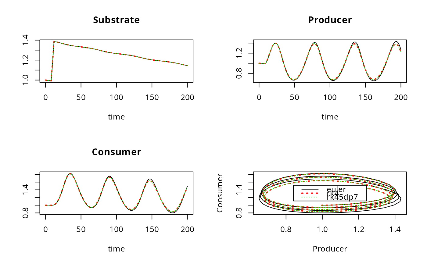
## =======================================================================
## Example: Resource-producer-consumer Lotka-Volterra model
## =======================================================================

## Notes:
## - Parameters are a list, names accessible via "with" function
## - Function sigimp passed as an argument (input) to model
##  (see also ode and lsoda examples)

SPCmod <- function(t, x, parms, input)  {
  with(as.list(c(parms, x)), {
    import <- input(t)
    dS <- import - b*S*P + g*C    # substrate
    dP <- c*S*P  - d*C*P          # producer
    dC <- e*P*C  - f*C            # consumer
    res <- c(dS, dP, dC)
    list(res)
  })
}

## The parameters
parms <- c(b = 0.001, c = 0.1, d = 0.1, e = 0.1, f = 0.1, g = 0.0)

## vector of timesteps
times <- seq(0, 200, length = 101)

## external signal with rectangle impulse
signal <- data.frame(times = times,
                     import = rep(0, length(times)))

signal$import[signal$times >= 10 & signal$times <= 11] <- 0.2

sigimp <- approxfun(signal$times, signal$import, rule = 2)

## Start values for steady state
xstart <- c(S = 1, P = 1, C = 1)

## Euler method
out1  <- rk(xstart, times, SPCmod, parms, hini = 0.1,
            input = sigimp, method = "euler")

## classical Runge-Kutta 4th order
out2 <- rk(xstart, times, SPCmod, parms, hini = 1,
           input = sigimp, method = "rk4")

## Dormand-Prince method of order 5(4)
out3 <- rk(xstart, times, SPCmod, parms, hmax = 1,
           input = sigimp, method = "rk45dp7")

mf <- par("mfrow")
## deSolve plot method for comparing scenarios
plot(out1, out2, out3, which = c("S", "P", "C"),
     main = c ("Substrate", "Producer", "Consumer"),
     col =c("black", "red", "green"),
     lty = c("solid", "dotted", "dotted"), lwd = c(1, 2, 1))

## user-specified plot function
plot (out1[,"P"], out1[,"C"], type = "l", xlab = "Producer", ylab = "Consumer")
lines(out2[,"P"], out2[,"C"], col = "red",   lty = "dotted", lwd = 2)
lines(out3[,"P"], out3[,"C"], col = "green", lty = "dotted")

legend("center", legend = c("euler", "rk4", "rk45dp7"),
  lty = c(1, 3, 3), lwd = c(1, 2, 1),
  col = c("black", "red", "green"))

par(mfrow = mf)