Solver for Ordinary Differential Equations (ODE), Switching Automatically Between Stiff and Non-stiff Methods

Solving initial value problems for stiff or non-stiff systems of first-order ordinary differential equations (ODEs).

The R function lsoda provides an interface to the FORTRAN ODE solver of the same name, written by Linda R. Petzold and Alan C. Hindmarsh.

The system of ODE's is written as an R function (which may, of course, use .C, .Fortran, .Call, etc., to call foreign code) or be defined in compiled code that has been dynamically loaded. A vector of parameters is passed to the ODEs, so the solver may be used as part of a modeling package for ODEs, or for parameter estimation using any appropriate modeling tool for non-linear models in R such as optim, nls, nlm or nlme

lsoda differs from the other integrators (except lsodar) in that it switches automatically between stiff and nonstiff methods. This means that the user does not have to determine whether the problem is stiff or not, and the solver will automatically choose the appropriate method. It always starts with the nonstiff method.

Usage

lsoda(y, times, func, parms, rtol = 1e-6, atol = 1e-6,
  jacfunc = NULL, jactype = "fullint", rootfunc = NULL,
  verbose = FALSE, nroot = 0, tcrit = NULL,
  hmin = 0, hmax = NULL, hini = 0, ynames = TRUE,
  maxordn = 12, maxords = 5, bandup = NULL, banddown = NULL,
  maxsteps = 5000, dllname = NULL, initfunc = dllname,
  initpar = parms, rpar = NULL, ipar = NULL, nout = 0,
  outnames = NULL, forcings = NULL, initforc = NULL,
  fcontrol = NULL, events = NULL, lags = NULL,...)

Arguments

y

the initial (state) values for the ODE system. If y has a name attribute, the names will be used to label the output matrix.

times

times at which explicit estimates for y are desired. The first value in times must be the initial time.

func

either an R-function that computes the values of the derivatives in the ODE system (the model definition) at time t, or a character string giving the name of a compiled function in a dynamically loaded shared library, or a list of symbols returned by checkDLL.

If func is an R-function, it must be defined as: func <- function(t, y, parms,...). t is the current time point in the integration, y is the current estimate of the variables in the ODE system. If the initial values y has a names attribute, the names will be available inside func. parms is a vector or list of parameters; ... (optional) are any other arguments passed to the function.

The return value of func should be a list, whose first element is a vector containing the derivatives of y with respect to time, and whose next elements are global values that are required at each point in times. The derivatives must be specified in the same order as the state variables y.

If func is a string, then dllname must give the name of the shared library (without extension) which must be loaded before lsoda() is called. See package vignette "compiledCode" for more details.

func can also be a list of symbols returned by checkDLL to avoid overhead from repeated internal calls to this function. It is an experimental feature for special situations, when a small compiled model with a low number of integration steps is repeatedly called. It is currently only available for the lsoda solver, see example.

parms

vector or list of parameters used in func or jacfunc.

rtol

relative error tolerance, either a scalar or an array as long as y. See details.

atol

absolute error tolerance, either a scalar or an array as long as y. See details.

jacfunc

if not NULL, an R function, that computes the Jacobian of the system of differential equations $\partial\dot{y}_i/\partial y_j$, or a string giving the name of a function or subroutine in dllname that computes the Jacobian (see vignette "compiledCode" for more about this option).

In some circumstances, supplying jacfunc can speed up the computations, if the system is stiff. The R calling sequence for jacfunc is identical to that of func.

If the Jacobian is a full matrix, jacfunc should return a matrix $\partial\dot{y}/\partial y$, where the ith row contains the derivative of $dy_i/dt$ with respect to $y_j$, or a vector containing the matrix elements by columns (the way R and FORTRAN store matrices).

If the Jacobian is banded, jacfunc should return a matrix containing only the nonzero bands of the Jacobian, rotated row-wise. See first example of lsode.

jactype

the structure of the Jacobian, one of "fullint", "fullusr", "bandusr" or "bandint" - either full or banded and estimated internally or by user.

rootfunc

if not NULL, an R function that computes the function whose root has to be estimated or a string giving the name of a function or subroutine in dllname that computes the root function. The R calling sequence for rootfunc is identical to that of func. rootfunc should return a vector with the function values whose root is sought. When rootfunc is provided, then lsodar will be called.

verbose

if TRUE: full output to the screen, e.g. will print the diagnostiscs of the integration - see details.

nroot

only used if dllname is specified: the number of constraint functions whose roots are desired during the integration; if rootfunc is an R-function, the solver estimates the number of roots.

tcrit

if not NULL, then lsoda cannot integrate past tcrit. The FORTRAN routine lsoda overshoots its targets (times points in the vector times), and interpolates values for the desired time points. If there is a time beyond which integration should not proceed (perhaps because of a singularity), that should be provided in tcrit.

hmin

an optional minimum value of the integration stepsize. In special situations this parameter may speed up computations with the cost of precision. Don't use hmin if you don't know why!

hmax

an optional maximum value of the integration stepsize. If not specified, hmax is set to the largest difference in times, to avoid that the simulation possibly ignores short-term events. If 0, no maximal size is specified.

hini

initial step size to be attempted; if 0, the initial step size is determined by the solver.

ynames

logical, if FALSE: names of state variables are not passed to function func; this may speed up the simulation especially for large models.

maxordn

the maximum order to be allowed in case the method is non-stiff. Should be <= 12. Reduce maxord to save storage space.

maxords

the maximum order to be allowed in case the method is stiff. Should be <= 5. Reduce maxord to save storage space.

bandup

number of non-zero bands above the diagonal, in case the Jacobian is banded.

banddown

number of non-zero bands below the diagonal, in case the Jacobian is banded.

maxsteps

maximal number of steps per output interval taken by the solver.

dllname

a string giving the name of the shared library (without extension) that contains all the compiled function or subroutine definitions refered to in func and jacfunc. See package vignette "compiledCode".

initfunc

if not NULL, the name of the initialisation function (which initialises values of parameters), as provided in dllname. See package vignette "compiledCode".

initpar

only when dllname is specified and an initialisation function initfunc is in the dll: the parameters passed to the initialiser, to initialise the common blocks (FORTRAN) or global variables (C, C++).

rpar

only when dllname is specified: a vector with double precision values passed to the dll-functions whose names are specified by func and jacfunc.

ipar

only when dllname is specified: a vector with integer values passed to the dll-functions whose names are specified by func and jacfunc.

nout

only used if dllname is specified and the model is defined in compiled code: the number of output variables calculated in the compiled function func, present in the shared library. Note: it is not automatically checked whether this is indeed the number of output variables calculated in the dll - you have to perform this check in the code. See package vignette "compiledCode".

outnames

only used if dllname is specified and nout > 0: the names of output variables calculated in the compiled function func, present in the shared library. These names will be used to label the output matrix.

forcings

only used if dllname is specified: a list with the forcing function data sets, each present as a two-columned matrix, with (time,value); interpolation outside the interval [min(times), max(times)] is done by taking the value at the closest data extreme.

See forcings or package vignette "compiledCode".

initforc

if not NULL, the name of the forcing function initialisation function, as provided in dllname. It MUST be present if forcings has been given a value. See forcings or package vignette "compiledCode".

fcontrol

A list of control parameters for the forcing functions. See forcings or vignette compiledCode.

events

A matrix or data frame that specifies events, i.e. when the value of a state variable is suddenly changed. See events for more information.

lags

A list that specifies timelags, i.e. the number of steps that has to be kept. To be used for delay differential equations. See timelags, dede for more information.

...

additional arguments passed to func and jacfunc allowing this to be a generic function.

Value

A matrix of class deSolve with up to as many rows as elements in times and as many columns as elements in y plus the number of "global" values returned in the next elements of the return from func, plus and additional column for the time value. There will be a row for each element in times unless the FORTRAN routine `lsoda' returns with an unrecoverable error. If y has a names attribute, it will be used to label the columns of the output value.

Author

R. Woodrow Setzer <setzer.woodrow@epa.gov>

References

Hindmarsh, Alan C. (1983) ODEPACK, A Systematized Collection of ODE Solvers; in p.55–64 of Stepleman, R.W. et al.[ed.] (1983) Scientific Computing, North-Holland, Amsterdam.

Petzold, Linda R. (1983) Automatic Selection of Methods for Solving Stiff and Nonstiff Systems of Ordinary Differential Equations. Siam J. Sci. Stat. Comput. 4, 136–148. doi:10.1137/0904010

Netlib: https://netlib.org

Details

All the hard work is done by the FORTRAN subroutine lsoda, whose documentation should be consulted for details (it is included as comments in the source file src/opkdmain.f). The implementation is based on the 12 November 2003 version of lsoda, from Netlib.

lsoda switches automatically between stiff and nonstiff methods. This means that the user does not have to determine whether the problem is stiff or not, and the solver will automatically choose the appropriate method. It always starts with the nonstiff method.

The form of the Jacobian can be specified by jactype which can take the following values:

"fullint": a full Jacobian, calculated internally by lsoda, the default,
"fullusr": a full Jacobian, specified by user function jacfunc,
"bandusr": a banded Jacobian, specified by user function jacfunc the size of the bands specified by bandup and banddown,
"bandint": banded Jacobian, calculated by lsoda; the size of the bands specified by bandup and banddown.

If jactype = "fullusr" or "bandusr" then the user must supply a subroutine jacfunc.

The following description of error control is adapted from the documentation of the lsoda source code (input arguments rtol and atol, above):

The input parameters rtol, and atol determine the error control performed by the solver. The solver will control the vector e of estimated local errors in y, according to an inequality of the form max-norm of ( e/ewt ) $\leq$ 1, where ewt is a vector of positive error weights. The values of rtol and atol should all be non-negative. The form of ewt is:

$$\mathbf{rtol} \times \mathrm{abs}(\mathbf{y}) + \mathbf{atol}$$

where multiplication of two vectors is element-by-element.

If the request for precision exceeds the capabilities of the machine, the FORTRAN subroutine lsoda will return an error code; under some circumstances, the R function lsoda will attempt a reasonable reduction of precision in order to get an answer. It will write a warning if it does so.

The diagnostics of the integration can be printed to screen by calling diagnostics. If verbose = TRUE, the diagnostics will written to the screen at the end of the integration.

See vignette("deSolve") for an explanation of each element in the vectors containing the diagnostic properties and how to directly access them.

Models may be defined in compiled C or FORTRAN code, as well as in an R-function. See package vignette "compiledCode" for details.

More information about models defined in compiled code is in the package vignette ("compiledCode"); information about linking forcing functions to compiled code is in forcings.

Examples in both C and FORTRAN are in the dynload subdirectory of the deSolve package directory.

Note

The demo directory contains some examples of using gnls to estimate parameters in a dynamic model.

Examples

## =======================================================================
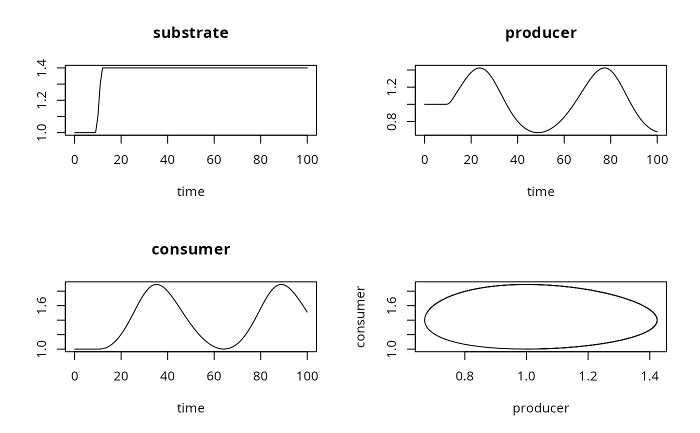
## Example 1:
##   A simple resource limited Lotka-Volterra-Model
##
## Note:
## 1. parameter and state variable names made
##    accessible via "with" function
## 2. function sigimp accessible through lexical scoping
##    (see also ode and rk examples)
## =======================================================================

SPCmod <- function(t, x, parms) {
  with(as.list(c(parms, x)), {
    import <- sigimp(t)
    dS <- import - b*S*P + g*C     #substrate
    dP <- c*S*P  - d*C*P           #producer
    dC <- e*P*C  - f*C             #consumer
    res <- c(dS, dP, dC)
    list(res)
  })
}

## Parameters
parms  <- c(b = 0.0, c = 0.1, d = 0.1, e = 0.1, f = 0.1, g = 0.0)

## vector of timesteps
times  <- seq(0, 100, length = 101)

## external signal with rectangle impulse
signal <- as.data.frame(list(times = times,
                            import = rep(0,length(times))))

signal$import[signal$times >= 10 & signal$times <= 11] <- 0.2

sigimp <- approxfun(signal$times, signal$import, rule = 2)


## Start values for steady state
y <- xstart <- c(S = 1, P = 1, C = 1)

## Solving
out <-  lsoda(xstart, times, SPCmod, parms)

## Plotting
mf <- par("mfrow")
plot(out, main = c("substrate", "producer", "consumer"))
plot(out[,"P"], out[,"C"], type = "l", xlab = "producer", ylab = "consumer")

par(mfrow = mf)

## =======================================================================
## Example 2:
##  from lsoda source code
## =======================================================================

## names makes this easier to read, but may slow down execution.
parms   <- c(k1 = 0.04, k2 = 1e4, k3 = 3e7)
my.atol <- c(1e-6,  1e-10,  1e-6)
times   <- c(0,4 * 10^(-1:10))

lsexamp <- function(t, y, p) {
  yd1 <- -p["k1"] * y[1] + p["k2"] * y[2]*y[3]
  yd3 <- p["k3"] * y[2]^2
  list(c(yd1, -yd1-yd3, yd3), c(massbalance = sum(y)))
}

exampjac <- function(t, y, p) {
  matrix(c(-p["k1"],     p["k1"],       0,

            p["k2"]*y[3],
          - p["k2"]*y[3] - 2*p["k3"]*y[2],
                           2*p["k3"]*y[2],

          p["k2"]*y[2],  -p["k2"]*y[2],  0
          ), 3, 3)
}


## measure speed (here and below)
system.time(
  out <- lsoda(c(1, 0, 0), times, lsexamp, parms, rtol = 1e-4,
           atol = my.atol, hmax = Inf)
)
#>    user  system elapsed 
#>   0.005   0.000   0.005 
out
#>     time            1            2          3 massbalance
#> 1  0e+00 1.000000e+00 0.000000e+00 0.00000000           1
#> 2  4e-01 9.851712e-01 3.386380e-05 0.01479493           1
#> 3  4e+00 9.055333e-01 2.240655e-05 0.09444430           1
#> 4  4e+01 7.158403e-01 9.186334e-06 0.28415047           1
#> 5  4e+02 4.505250e-01 3.222964e-06 0.54947175           1
#> 6  4e+03 1.831976e-01 8.941774e-07 0.81680155           1
#> 7  4e+04 3.898729e-02 1.621940e-07 0.96101254           1
#> 8  4e+05 4.936362e-03 1.984221e-08 0.99506362           1
#> 9  4e+06 5.161832e-04 2.065786e-09 0.99948381           1
#> 10 4e+07 5.179808e-05 2.072029e-10 0.99994820           1
#> 11 4e+08 5.283591e-06 2.113447e-11 0.99999472           1
#> 12 4e+09 4.658821e-07 1.863529e-12 0.99999953           1
#> 13 4e+10 1.426830e-08 5.707325e-14 0.99999999           1

## This is what the authors of lsoda got for the example:

## the output of this program (on a cdc-7600 in single precision)
## is as follows..
##
## at t =  4.0000e-01   y =  9.851712e-01  3.386380e-05  1.479493e-02
## at t =  4.0000e+00   y =  9.055333e-01  2.240655e-05  9.444430e-02
## at t =  4.0000e+01   y =  7.158403e-01  9.186334e-06  2.841505e-01
## at t =  4.0000e+02   y =  4.505250e-01  3.222964e-06  5.494717e-01
## at t =  4.0000e+03   y =  1.831975e-01  8.941774e-07  8.168016e-01
## at t =  4.0000e+04   y =  3.898730e-02  1.621940e-07  9.610125e-01
## at t =  4.0000e+05   y =  4.936363e-03  1.984221e-08  9.950636e-01
## at t =  4.0000e+06   y =  5.161831e-04  2.065786e-09  9.994838e-01
## at t =  4.0000e+07   y =  5.179817e-05  2.072032e-10  9.999482e-01
## at t =  4.0000e+08   y =  5.283401e-06  2.113371e-11  9.999947e-01
## at t =  4.0000e+09   y =  4.659031e-07  1.863613e-12  9.999995e-01
## at t =  4.0000e+10   y =  1.404280e-08  5.617126e-14  1.000000e+00

## Using the analytic Jacobian speeds up execution a little :

system.time(
  outJ <- lsoda(c(1, 0, 0), times, lsexamp, parms, rtol = 1e-4,
            atol = my.atol, jacfunc = exampjac, jactype = "fullusr", hmax = Inf)
)
#>    user  system elapsed 
#>   0.009   0.000   0.010 

all.equal(as.data.frame(out), as.data.frame(outJ)) # TRUE
#> [1] TRUE
diagnostics(out)
#> 
#> --------------------
#> lsoda return code
#> --------------------
#> 
#>   return code (idid) =  2 
#>   Integration was successful.
#> 
#> --------------------
#> INTEGER values
#> --------------------
#> 
#>   1 The return code : 2 
#>   2 The number of steps taken for the problem so far: 361 
#>   3 The number of function evaluations for the problem so far: 693 
#>   5 The method order last used (successfully): 1 
#>   6 The order of the method to be attempted on the next step: 1 
#>   7 If return flag =-4,-5: the largest component in error vector 0 
#>   8 The length of the real work array actually required: 68 
#>   9 The length of the integer work array actually required: 23 
#>  14 The number of Jacobian evaluations and LU decompositions so far: 64 
#>  15 The method indicator for the last succesful step,
#>            1=adams (nonstiff), 2= bdf (stiff): 2 
#>  16 The current method indicator to be attempted on the next step,
#>            1=adams (nonstiff), 2= bdf (stiff): 2 
#>  
#> --------------------
#> RSTATE values
#> --------------------
#> 
#>   1 The step size in t last used (successfully): 44020830000 
#>   2 The step size to be attempted on the next step: 44020830000 
#>   3 The current value of the independent variable which the solver has reached: 64822650000 
#>   4 Tolerance scale factor > 1.0 computed when requesting too much accuracy: 0 
#>   5 The value of t at the time of the last method switch, if any: 0.006009229 
#>  
diagnostics(outJ) # shows what lsoda did internally
#> 
#> --------------------
#> lsoda return code
#> --------------------
#> 
#>   return code (idid) =  2 
#>   Integration was successful.
#> 
#> --------------------
#> INTEGER values
#> --------------------
#> 
#>   1 The return code : 2 
#>   2 The number of steps taken for the problem so far: 361 
#>   3 The number of function evaluations for the problem so far: 501 
#>   5 The method order last used (successfully): 1 
#>   6 The order of the method to be attempted on the next step: 1 
#>   7 If return flag =-4,-5: the largest component in error vector 0 
#>   8 The length of the real work array actually required: 68 
#>   9 The length of the integer work array actually required: 23 
#>  14 The number of Jacobian evaluations and LU decompositions so far: 64 
#>  15 The method indicator for the last succesful step,
#>            1=adams (nonstiff), 2= bdf (stiff): 2 
#>  16 The current method indicator to be attempted on the next step,
#>            1=adams (nonstiff), 2= bdf (stiff): 2 
#>  
#> --------------------
#> RSTATE values
#> --------------------
#> 
#>   1 The step size in t last used (successfully): 44025240000 
#>   2 The step size to be attempted on the next step: 44025240000 
#>   3 The current value of the independent variable which the solver has reached: 64828600000 
#>   4 Tolerance scale factor > 1.0 computed when requesting too much accuracy: 0 
#>   5 The value of t at the time of the last method switch, if any: 0.006009229 
#>