Data and Examples from Greene (2003)
Greene2003.RdThis manual page collects a list of examples from the book. Some solutions might not be exact and the list is certainly not complete. If you have suggestions for improvement (preferably in the form of code), please contact the package maintainer.
References
Greene, W.H. (2003). Econometric Analysis, 5th edition. Upper Saddle River, NJ: Prentice Hall. URL https://pages.stern.nyu.edu/~wgreene/Text/tables/tablelist5.htm.
See also
Affairs, BondYield, CreditCard,
Electricity1955, Electricity1970, Equipment,
Grunfeld, KleinI, Longley,
ManufactCosts, MarkPound, Municipalities,
ProgramEffectiveness, PSID1976, SIC33,
ShipAccidents, StrikeDuration, TechChange,
TravelMode, UKInflation, USConsump1950,
USConsump1979, USGasG, USAirlines,
USInvest, USMacroG, USMoney
Examples
#> Loading required namespace: sampleSelection
# \donttest{
#####################################
## US consumption data (1970-1979) ##
#####################################
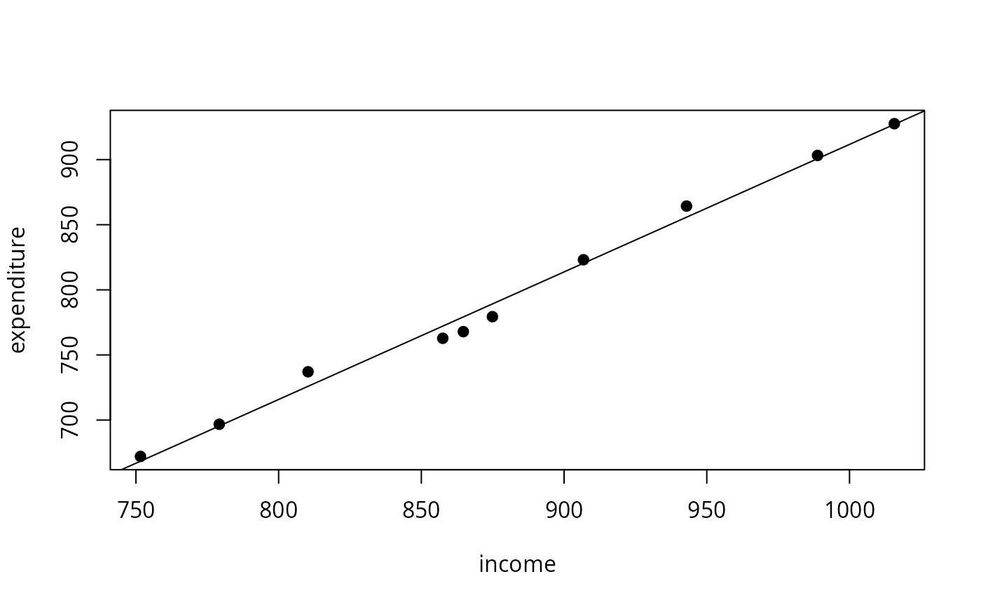
## Example 1.1
data("USConsump1979", package = "AER")
plot(expenditure ~ income, data = as.data.frame(USConsump1979), pch = 19)
fm <- lm(expenditure ~ income, data = as.data.frame(USConsump1979))
summary(fm)
#>
#> Call:
#> lm(formula = expenditure ~ income, data = as.data.frame(USConsump1979))
#>
#> Residuals:
#> Min 1Q Median 3Q Max
#> -11.291 -6.871 1.909 3.418 11.181
#>
#> Coefficients:
#> Estimate Std. Error t value Pr(>|t|)
#> (Intercept) -67.58065 27.91071 -2.421 0.0418 *
#> income 0.97927 0.03161 30.983 1.28e-09 ***
#> ---
#> Signif. codes: 0 ‘***’ 0.001 ‘**’ 0.01 ‘*’ 0.05 ‘.’ 0.1 ‘ ’ 1
#>
#> Residual standard error: 8.193 on 8 degrees of freedom
#> Multiple R-squared: 0.9917, Adjusted R-squared: 0.9907
#> F-statistic: 959.9 on 1 and 8 DF, p-value: 1.28e-09
#>
abline(fm)
 #####################################
## US consumption data (1940-1950) ##
#####################################
## data
data("USConsump1950", package = "AER")
usc <- as.data.frame(USConsump1950)
usc$war <- factor(usc$war, labels = c("no", "yes"))
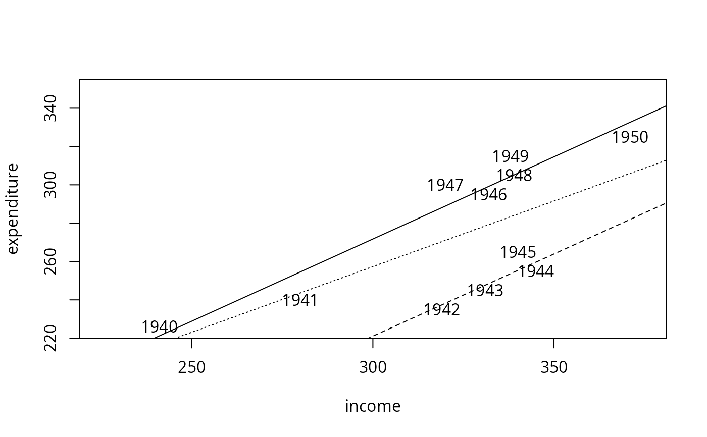
## Example 2.1
plot(expenditure ~ income, data = usc, type = "n", xlim = c(225, 375), ylim = c(225, 350))
with(usc, text(income, expenditure, time(USConsump1950)))
## single model
fm <- lm(expenditure ~ income, data = usc)
summary(fm)
#>
#> Call:
#> lm(formula = expenditure ~ income, data = usc)
#>
#> Residuals:
#> Min 1Q Median 3Q Max
#> -35.347 -26.440 9.068 20.000 31.642
#>
#> Coefficients:
#> Estimate Std. Error t value Pr(>|t|)
#> (Intercept) 51.8951 80.8440 0.642 0.5369
#> income 0.6848 0.2488 2.753 0.0224 *
#> ---
#> Signif. codes: 0 ‘***’ 0.001 ‘**’ 0.01 ‘*’ 0.05 ‘.’ 0.1 ‘ ’ 1
#>
#> Residual standard error: 27.59 on 9 degrees of freedom
#> Multiple R-squared: 0.4571, Adjusted R-squared: 0.3968
#> F-statistic: 7.579 on 1 and 9 DF, p-value: 0.02237
#>
## different intercepts for war yes/no
fm2 <- lm(expenditure ~ income + war, data = usc)
summary(fm2)
#>
#> Call:
#> lm(formula = expenditure ~ income + war, data = usc)
#>
#> Residuals:
#> Min 1Q Median 3Q Max
#> -14.598 -4.418 -2.352 7.242 11.101
#>
#> Coefficients:
#> Estimate Std. Error t value Pr(>|t|)
#> (Intercept) 14.49540 27.29948 0.531 0.61
#> income 0.85751 0.08534 10.048 8.19e-06 ***
#> waryes -50.68974 5.93237 -8.545 2.71e-05 ***
#> ---
#> Signif. codes: 0 ‘***’ 0.001 ‘**’ 0.01 ‘*’ 0.05 ‘.’ 0.1 ‘ ’ 1
#>
#> Residual standard error: 9.195 on 8 degrees of freedom
#> Multiple R-squared: 0.9464, Adjusted R-squared: 0.933
#> F-statistic: 70.61 on 2 and 8 DF, p-value: 8.26e-06
#>
## compare
anova(fm, fm2)
#> Analysis of Variance Table
#>
#> Model 1: expenditure ~ income
#> Model 2: expenditure ~ income + war
#> Res.Df RSS Df Sum of Sq F Pr(>F)
#> 1 9 6850.0
#> 2 8 676.5 1 6173.5 73.01 2.71e-05 ***
#> ---
#> Signif. codes: 0 ‘***’ 0.001 ‘**’ 0.01 ‘*’ 0.05 ‘.’ 0.1 ‘ ’ 1
## visualize
abline(fm, lty = 3)
abline(coef(fm2)[1:2])
abline(sum(coef(fm2)[c(1, 3)]), coef(fm2)[2], lty = 2)
#####################################
## US consumption data (1940-1950) ##
#####################################
## data
data("USConsump1950", package = "AER")
usc <- as.data.frame(USConsump1950)
usc$war <- factor(usc$war, labels = c("no", "yes"))
## Example 2.1
plot(expenditure ~ income, data = usc, type = "n", xlim = c(225, 375), ylim = c(225, 350))
with(usc, text(income, expenditure, time(USConsump1950)))
## single model
fm <- lm(expenditure ~ income, data = usc)
summary(fm)
#>
#> Call:
#> lm(formula = expenditure ~ income, data = usc)
#>
#> Residuals:
#> Min 1Q Median 3Q Max
#> -35.347 -26.440 9.068 20.000 31.642
#>
#> Coefficients:
#> Estimate Std. Error t value Pr(>|t|)
#> (Intercept) 51.8951 80.8440 0.642 0.5369
#> income 0.6848 0.2488 2.753 0.0224 *
#> ---
#> Signif. codes: 0 ‘***’ 0.001 ‘**’ 0.01 ‘*’ 0.05 ‘.’ 0.1 ‘ ’ 1
#>
#> Residual standard error: 27.59 on 9 degrees of freedom
#> Multiple R-squared: 0.4571, Adjusted R-squared: 0.3968
#> F-statistic: 7.579 on 1 and 9 DF, p-value: 0.02237
#>
## different intercepts for war yes/no
fm2 <- lm(expenditure ~ income + war, data = usc)
summary(fm2)
#>
#> Call:
#> lm(formula = expenditure ~ income + war, data = usc)
#>
#> Residuals:
#> Min 1Q Median 3Q Max
#> -14.598 -4.418 -2.352 7.242 11.101
#>
#> Coefficients:
#> Estimate Std. Error t value Pr(>|t|)
#> (Intercept) 14.49540 27.29948 0.531 0.61
#> income 0.85751 0.08534 10.048 8.19e-06 ***
#> waryes -50.68974 5.93237 -8.545 2.71e-05 ***
#> ---
#> Signif. codes: 0 ‘***’ 0.001 ‘**’ 0.01 ‘*’ 0.05 ‘.’ 0.1 ‘ ’ 1
#>
#> Residual standard error: 9.195 on 8 degrees of freedom
#> Multiple R-squared: 0.9464, Adjusted R-squared: 0.933
#> F-statistic: 70.61 on 2 and 8 DF, p-value: 8.26e-06
#>
## compare
anova(fm, fm2)
#> Analysis of Variance Table
#>
#> Model 1: expenditure ~ income
#> Model 2: expenditure ~ income + war
#> Res.Df RSS Df Sum of Sq F Pr(>F)
#> 1 9 6850.0
#> 2 8 676.5 1 6173.5 73.01 2.71e-05 ***
#> ---
#> Signif. codes: 0 ‘***’ 0.001 ‘**’ 0.01 ‘*’ 0.05 ‘.’ 0.1 ‘ ’ 1
## visualize
abline(fm, lty = 3)
abline(coef(fm2)[1:2])
abline(sum(coef(fm2)[c(1, 3)]), coef(fm2)[2], lty = 2)
 ## Example 3.2
summary(fm)$r.squared
#> [1] 0.4571345
summary(lm(expenditure ~ income, data = usc, subset = war == "no"))$r.squared
#> [1] 0.9369742
summary(fm2)$r.squared
#> [1] 0.9463904
########################
## US investment data ##
########################
data("USInvest", package = "AER")
## Chapter 3 in Greene (2003)
## transform (and round) data to match Table 3.1
us <- as.data.frame(USInvest)
us$invest <- round(0.1 * us$invest/us$price, digits = 3)
us$gnp <- round(0.1 * us$gnp/us$price, digits = 3)
us$inflation <- c(4.4, round(100 * diff(us$price)/us$price[-15], digits = 2))
us$trend <- 1:15
us <- us[, c(2, 6, 1, 4, 5)]
## p. 22-24
coef(lm(invest ~ trend + gnp, data = us))
#> (Intercept) trend gnp
#> -0.49459760 -0.01700063 0.64781939
coef(lm(invest ~ gnp, data = us))
#> (Intercept) gnp
#> -0.03333061 0.18388271
## Example 3.1, Table 3.2
cor(us)[1,-1]
#> trend gnp interest inflation
#> 0.7514213 0.8648613 0.5876756 0.4817416
pcor <- solve(cor(us))
dcor <- 1/sqrt(diag(pcor))
pcor <- (-pcor * (dcor %o% dcor))[1,-1]
## Table 3.4
fm <- lm(invest ~ trend + gnp + interest + inflation, data = us)
fm1 <- lm(invest ~ 1, data = us)
anova(fm1, fm)
#> Analysis of Variance Table
#>
#> Model 1: invest ~ 1
#> Model 2: invest ~ trend + gnp + interest + inflation
#> Res.Df RSS Df Sum of Sq F Pr(>F)
#> 1 14 0.0162736
#> 2 10 0.0004394 4 0.015834 90.089 8.417e-08 ***
#> ---
#> Signif. codes: 0 ‘***’ 0.001 ‘**’ 0.01 ‘*’ 0.05 ‘.’ 0.1 ‘ ’ 1
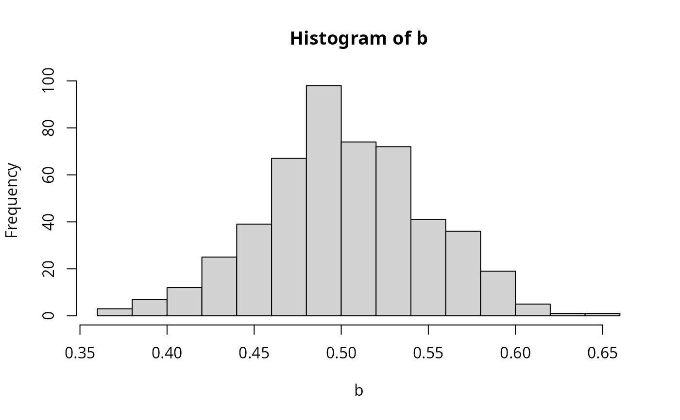
## Example 4.1
set.seed(123)
w <- rnorm(10000)
x <- rnorm(10000)
eps <- 0.5 * w
y <- 0.5 + 0.5 * x + eps
b <- rep(0, 500)
for(i in 1:500) {
ix <- sample(1:10000, 100)
b[i] <- lm.fit(cbind(1, x[ix]), y[ix])$coef[2]
}
hist(b, breaks = 20, col = "lightgray")
## Example 3.2
summary(fm)$r.squared
#> [1] 0.4571345
summary(lm(expenditure ~ income, data = usc, subset = war == "no"))$r.squared
#> [1] 0.9369742
summary(fm2)$r.squared
#> [1] 0.9463904
########################
## US investment data ##
########################
data("USInvest", package = "AER")
## Chapter 3 in Greene (2003)
## transform (and round) data to match Table 3.1
us <- as.data.frame(USInvest)
us$invest <- round(0.1 * us$invest/us$price, digits = 3)
us$gnp <- round(0.1 * us$gnp/us$price, digits = 3)
us$inflation <- c(4.4, round(100 * diff(us$price)/us$price[-15], digits = 2))
us$trend <- 1:15
us <- us[, c(2, 6, 1, 4, 5)]
## p. 22-24
coef(lm(invest ~ trend + gnp, data = us))
#> (Intercept) trend gnp
#> -0.49459760 -0.01700063 0.64781939
coef(lm(invest ~ gnp, data = us))
#> (Intercept) gnp
#> -0.03333061 0.18388271
## Example 3.1, Table 3.2
cor(us)[1,-1]
#> trend gnp interest inflation
#> 0.7514213 0.8648613 0.5876756 0.4817416
pcor <- solve(cor(us))
dcor <- 1/sqrt(diag(pcor))
pcor <- (-pcor * (dcor %o% dcor))[1,-1]
## Table 3.4
fm <- lm(invest ~ trend + gnp + interest + inflation, data = us)
fm1 <- lm(invest ~ 1, data = us)
anova(fm1, fm)
#> Analysis of Variance Table
#>
#> Model 1: invest ~ 1
#> Model 2: invest ~ trend + gnp + interest + inflation
#> Res.Df RSS Df Sum of Sq F Pr(>F)
#> 1 14 0.0162736
#> 2 10 0.0004394 4 0.015834 90.089 8.417e-08 ***
#> ---
#> Signif. codes: 0 ‘***’ 0.001 ‘**’ 0.01 ‘*’ 0.05 ‘.’ 0.1 ‘ ’ 1
## Example 4.1
set.seed(123)
w <- rnorm(10000)
x <- rnorm(10000)
eps <- 0.5 * w
y <- 0.5 + 0.5 * x + eps
b <- rep(0, 500)
for(i in 1:500) {
ix <- sample(1:10000, 100)
b[i] <- lm.fit(cbind(1, x[ix]), y[ix])$coef[2]
}
hist(b, breaks = 20, col = "lightgray")
 ###############################
## Longley's regression data ##
###############################
## package and data
data("Longley", package = "AER")
library("dynlm")
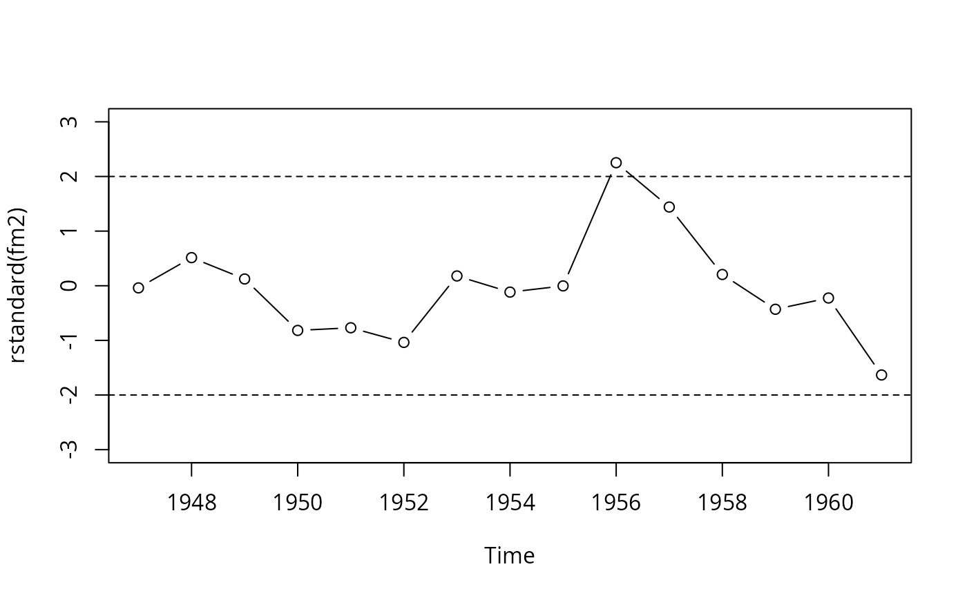
## Example 4.6
fm1 <- dynlm(employment ~ time(employment) + price + gnp + armedforces,
data = Longley)
fm2 <- update(fm1, end = 1961)
cbind(coef(fm2), coef(fm1))
#> [,1] [,2]
#> (Intercept) 1.459415e+06 1.169088e+06
#> time(employment) -7.217561e+02 -5.764643e+02
#> price -1.811230e+02 -1.976807e+01
#> gnp 9.106778e-02 6.439397e-02
#> armedforces -7.493705e-02 -1.014525e-02
## Figure 4.3
plot(rstandard(fm2), type = "b", ylim = c(-3, 3))
abline(h = c(-2, 2), lty = 2)
###############################
## Longley's regression data ##
###############################
## package and data
data("Longley", package = "AER")
library("dynlm")
## Example 4.6
fm1 <- dynlm(employment ~ time(employment) + price + gnp + armedforces,
data = Longley)
fm2 <- update(fm1, end = 1961)
cbind(coef(fm2), coef(fm1))
#> [,1] [,2]
#> (Intercept) 1.459415e+06 1.169088e+06
#> time(employment) -7.217561e+02 -5.764643e+02
#> price -1.811230e+02 -1.976807e+01
#> gnp 9.106778e-02 6.439397e-02
#> armedforces -7.493705e-02 -1.014525e-02
## Figure 4.3
plot(rstandard(fm2), type = "b", ylim = c(-3, 3))
abline(h = c(-2, 2), lty = 2)
 #########################################
## US gasoline market data (1960-1995) ##
#########################################
## data
data("USGasG", package = "AER")
## Greene (2003)
## Example 2.3
fm <- lm(log(gas/population) ~ log(price) + log(income) + log(newcar) + log(usedcar),
data = as.data.frame(USGasG))
summary(fm)
#>
#> Call:
#> lm(formula = log(gas/population) ~ log(price) + log(income) +
#> log(newcar) + log(usedcar), data = as.data.frame(USGasG))
#>
#> Residuals:
#> Min 1Q Median 3Q Max
#> -0.065042 -0.018842 0.001528 0.020786 0.058084
#>
#> Coefficients:
#> Estimate Std. Error t value Pr(>|t|)
#> (Intercept) -12.34184 0.67489 -18.287 <2e-16 ***
#> log(price) -0.05910 0.03248 -1.819 0.0786 .
#> log(income) 1.37340 0.07563 18.160 <2e-16 ***
#> log(newcar) -0.12680 0.12699 -0.998 0.3258
#> log(usedcar) -0.11871 0.08134 -1.459 0.1545
#> ---
#> Signif. codes: 0 ‘***’ 0.001 ‘**’ 0.01 ‘*’ 0.05 ‘.’ 0.1 ‘ ’ 1
#>
#> Residual standard error: 0.03304 on 31 degrees of freedom
#> Multiple R-squared: 0.958, Adjusted R-squared: 0.9526
#> F-statistic: 176.7 on 4 and 31 DF, p-value: < 2.2e-16
#>
## Example 4.4
## estimates and standard errors (note different offset for intercept)
coef(fm)
#> (Intercept) log(price) log(income) log(newcar) log(usedcar)
#> -12.34184054 -0.05909513 1.37339912 -0.12679667 -0.11870847
sqrt(diag(vcov(fm)))
#> (Intercept) log(price) log(income) log(newcar) log(usedcar)
#> 0.67489471 0.03248496 0.07562767 0.12699351 0.08133710
## confidence interval
confint(fm, parm = "log(income)")
#> 2.5 % 97.5 %
#> log(income) 1.219155 1.527643
## test linear hypothesis
linearHypothesis(fm, "log(income) = 1")
#>
#> Linear hypothesis test:
#> log(income) = 1
#>
#> Model 1: restricted model
#> Model 2: log(gas/population) ~ log(price) + log(income) + log(newcar) +
#> log(usedcar)
#>
#> Res.Df RSS Df Sum of Sq F Pr(>F)
#> 1 32 0.060445
#> 2 31 0.033837 1 0.026608 24.377 2.57e-05 ***
#> ---
#> Signif. codes: 0 ‘***’ 0.001 ‘**’ 0.01 ‘*’ 0.05 ‘.’ 0.1 ‘ ’ 1
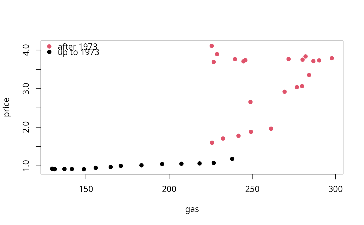
## Figure 7.5
plot(price ~ gas, data = as.data.frame(USGasG), pch = 19,
col = (time(USGasG) > 1973) + 1)
legend("topleft", legend = c("after 1973", "up to 1973"), pch = 19, col = 2:1, bty = "n")
#########################################
## US gasoline market data (1960-1995) ##
#########################################
## data
data("USGasG", package = "AER")
## Greene (2003)
## Example 2.3
fm <- lm(log(gas/population) ~ log(price) + log(income) + log(newcar) + log(usedcar),
data = as.data.frame(USGasG))
summary(fm)
#>
#> Call:
#> lm(formula = log(gas/population) ~ log(price) + log(income) +
#> log(newcar) + log(usedcar), data = as.data.frame(USGasG))
#>
#> Residuals:
#> Min 1Q Median 3Q Max
#> -0.065042 -0.018842 0.001528 0.020786 0.058084
#>
#> Coefficients:
#> Estimate Std. Error t value Pr(>|t|)
#> (Intercept) -12.34184 0.67489 -18.287 <2e-16 ***
#> log(price) -0.05910 0.03248 -1.819 0.0786 .
#> log(income) 1.37340 0.07563 18.160 <2e-16 ***
#> log(newcar) -0.12680 0.12699 -0.998 0.3258
#> log(usedcar) -0.11871 0.08134 -1.459 0.1545
#> ---
#> Signif. codes: 0 ‘***’ 0.001 ‘**’ 0.01 ‘*’ 0.05 ‘.’ 0.1 ‘ ’ 1
#>
#> Residual standard error: 0.03304 on 31 degrees of freedom
#> Multiple R-squared: 0.958, Adjusted R-squared: 0.9526
#> F-statistic: 176.7 on 4 and 31 DF, p-value: < 2.2e-16
#>
## Example 4.4
## estimates and standard errors (note different offset for intercept)
coef(fm)
#> (Intercept) log(price) log(income) log(newcar) log(usedcar)
#> -12.34184054 -0.05909513 1.37339912 -0.12679667 -0.11870847
sqrt(diag(vcov(fm)))
#> (Intercept) log(price) log(income) log(newcar) log(usedcar)
#> 0.67489471 0.03248496 0.07562767 0.12699351 0.08133710
## confidence interval
confint(fm, parm = "log(income)")
#> 2.5 % 97.5 %
#> log(income) 1.219155 1.527643
## test linear hypothesis
linearHypothesis(fm, "log(income) = 1")
#>
#> Linear hypothesis test:
#> log(income) = 1
#>
#> Model 1: restricted model
#> Model 2: log(gas/population) ~ log(price) + log(income) + log(newcar) +
#> log(usedcar)
#>
#> Res.Df RSS Df Sum of Sq F Pr(>F)
#> 1 32 0.060445
#> 2 31 0.033837 1 0.026608 24.377 2.57e-05 ***
#> ---
#> Signif. codes: 0 ‘***’ 0.001 ‘**’ 0.01 ‘*’ 0.05 ‘.’ 0.1 ‘ ’ 1
## Figure 7.5
plot(price ~ gas, data = as.data.frame(USGasG), pch = 19,
col = (time(USGasG) > 1973) + 1)
legend("topleft", legend = c("after 1973", "up to 1973"), pch = 19, col = 2:1, bty = "n")
 ## Example 7.6
## re-used in Example 8.3
## linear time trend
ltrend <- 1:nrow(USGasG)
## shock factor
shock <- factor(time(USGasG) > 1973, levels = c(FALSE, TRUE), labels = c("before", "after"))
## 1960-1995
fm1 <- lm(log(gas/population) ~ log(income) + log(price) + log(newcar) + log(usedcar) + ltrend,
data = as.data.frame(USGasG))
summary(fm1)
#>
#> Call:
#> lm(formula = log(gas/population) ~ log(income) + log(price) +
#> log(newcar) + log(usedcar) + ltrend, data = as.data.frame(USGasG))
#>
#> Residuals:
#> Min 1Q Median 3Q Max
#> -0.055238 -0.017715 0.003659 0.016481 0.053522
#>
#> Coefficients:
#> Estimate Std. Error t value Pr(>|t|)
#> (Intercept) -17.385790 1.679289 -10.353 2.03e-11 ***
#> log(income) 1.954626 0.192854 10.135 3.34e-11 ***
#> log(price) -0.115530 0.033479 -3.451 0.00168 **
#> log(newcar) 0.205282 0.152019 1.350 0.18700
#> log(usedcar) -0.129274 0.071412 -1.810 0.08028 .
#> ltrend -0.019118 0.005957 -3.210 0.00316 **
#> ---
#> Signif. codes: 0 ‘***’ 0.001 ‘**’ 0.01 ‘*’ 0.05 ‘.’ 0.1 ‘ ’ 1
#>
#> Residual standard error: 0.02898 on 30 degrees of freedom
#> Multiple R-squared: 0.9687, Adjusted R-squared: 0.9635
#> F-statistic: 185.8 on 5 and 30 DF, p-value: < 2.2e-16
#>
## pooled
fm2 <- lm(
log(gas/population) ~ shock + log(income) + log(price) + log(newcar) + log(usedcar) + ltrend,
data = as.data.frame(USGasG))
summary(fm2)
#>
#> Call:
#> lm(formula = log(gas/population) ~ shock + log(income) + log(price) +
#> log(newcar) + log(usedcar) + ltrend, data = as.data.frame(USGasG))
#>
#> Residuals:
#> Min 1Q Median 3Q Max
#> -0.045360 -0.019697 0.003931 0.015112 0.047550
#>
#> Coefficients:
#> Estimate Std. Error t value Pr(>|t|)
#> (Intercept) -16.374402 1.456263 -11.244 4.33e-12 ***
#> shockafter 0.077311 0.021872 3.535 0.00139 **
#> log(income) 1.838167 0.167258 10.990 7.43e-12 ***
#> log(price) -0.178005 0.033508 -5.312 1.06e-05 ***
#> log(newcar) 0.209842 0.129267 1.623 0.11534
#> log(usedcar) -0.128132 0.060721 -2.110 0.04359 *
#> ltrend -0.016862 0.005105 -3.303 0.00255 **
#> ---
#> Signif. codes: 0 ‘***’ 0.001 ‘**’ 0.01 ‘*’ 0.05 ‘.’ 0.1 ‘ ’ 1
#>
#> Residual standard error: 0.02464 on 29 degrees of freedom
#> Multiple R-squared: 0.9781, Adjusted R-squared: 0.9736
#> F-statistic: 216.3 on 6 and 29 DF, p-value: < 2.2e-16
#>
## segmented
fm3 <- lm(
log(gas/population) ~ shock/(log(income) + log(price) + log(newcar) + log(usedcar) + ltrend),
data = as.data.frame(USGasG))
summary(fm3)
#>
#> Call:
#> lm(formula = log(gas/population) ~ shock/(log(income) + log(price) +
#> log(newcar) + log(usedcar) + ltrend), data = as.data.frame(USGasG))
#>
#> Residuals:
#> Min 1Q Median 3Q Max
#> -0.027349 -0.006332 0.001295 0.007159 0.022016
#>
#> Coefficients:
#> Estimate Std. Error t value Pr(>|t|)
#> (Intercept) -4.13439 5.03963 -0.820 0.420075
#> shockafter -4.74111 5.51576 -0.860 0.398538
#> shockbefore:log(income) 0.42400 0.57973 0.731 0.471633
#> shockafter:log(income) 1.01408 0.24904 4.072 0.000439 ***
#> shockbefore:log(price) 0.09455 0.24804 0.381 0.706427
#> shockafter:log(price) -0.24237 0.03490 -6.946 3.5e-07 ***
#> shockbefore:log(newcar) 0.58390 0.21670 2.695 0.012665 *
#> shockafter:log(newcar) 0.33017 0.15789 2.091 0.047277 *
#> shockbefore:log(usedcar) -0.33462 0.15215 -2.199 0.037738 *
#> shockafter:log(usedcar) -0.05537 0.04426 -1.251 0.222972
#> shockbefore:ltrend 0.02637 0.01762 1.497 0.147533
#> shockafter:ltrend -0.01262 0.00329 -3.835 0.000798 ***
#> ---
#> Signif. codes: 0 ‘***’ 0.001 ‘**’ 0.01 ‘*’ 0.05 ‘.’ 0.1 ‘ ’ 1
#>
#> Residual standard error: 0.01488 on 24 degrees of freedom
#> Multiple R-squared: 0.9934, Adjusted R-squared: 0.9904
#> F-statistic: 328.5 on 11 and 24 DF, p-value: < 2.2e-16
#>
## Chow test
anova(fm3, fm1)
#> Analysis of Variance Table
#>
#> Model 1: log(gas/population) ~ shock/(log(income) + log(price) + log(newcar) +
#> log(usedcar) + ltrend)
#> Model 2: log(gas/population) ~ log(income) + log(price) + log(newcar) +
#> log(usedcar) + ltrend
#> Res.Df RSS Df Sum of Sq F Pr(>F)
#> 1 24 0.0053144
#> 2 30 0.0251878 -6 -0.019873 14.958 4.595e-07 ***
#> ---
#> Signif. codes: 0 ‘***’ 0.001 ‘**’ 0.01 ‘*’ 0.05 ‘.’ 0.1 ‘ ’ 1
library("strucchange")
sctest(log(gas/population) ~ log(income) + log(price) + log(newcar) + log(usedcar) + ltrend,
data = USGasG, point = c(1973, 1), type = "Chow")
#>
#> Chow test
#>
#> data: log(gas/population) ~ log(income) + log(price) + log(newcar) + log(usedcar) + ltrend
#> F = 14.958, p-value = 4.595e-07
#>
## Recursive CUSUM test
rcus <- efp(log(gas/population) ~ log(income) + log(price) + log(newcar) + log(usedcar) + ltrend,
data = USGasG, type = "Rec-CUSUM")
plot(rcus)
## Example 7.6
## re-used in Example 8.3
## linear time trend
ltrend <- 1:nrow(USGasG)
## shock factor
shock <- factor(time(USGasG) > 1973, levels = c(FALSE, TRUE), labels = c("before", "after"))
## 1960-1995
fm1 <- lm(log(gas/population) ~ log(income) + log(price) + log(newcar) + log(usedcar) + ltrend,
data = as.data.frame(USGasG))
summary(fm1)
#>
#> Call:
#> lm(formula = log(gas/population) ~ log(income) + log(price) +
#> log(newcar) + log(usedcar) + ltrend, data = as.data.frame(USGasG))
#>
#> Residuals:
#> Min 1Q Median 3Q Max
#> -0.055238 -0.017715 0.003659 0.016481 0.053522
#>
#> Coefficients:
#> Estimate Std. Error t value Pr(>|t|)
#> (Intercept) -17.385790 1.679289 -10.353 2.03e-11 ***
#> log(income) 1.954626 0.192854 10.135 3.34e-11 ***
#> log(price) -0.115530 0.033479 -3.451 0.00168 **
#> log(newcar) 0.205282 0.152019 1.350 0.18700
#> log(usedcar) -0.129274 0.071412 -1.810 0.08028 .
#> ltrend -0.019118 0.005957 -3.210 0.00316 **
#> ---
#> Signif. codes: 0 ‘***’ 0.001 ‘**’ 0.01 ‘*’ 0.05 ‘.’ 0.1 ‘ ’ 1
#>
#> Residual standard error: 0.02898 on 30 degrees of freedom
#> Multiple R-squared: 0.9687, Adjusted R-squared: 0.9635
#> F-statistic: 185.8 on 5 and 30 DF, p-value: < 2.2e-16
#>
## pooled
fm2 <- lm(
log(gas/population) ~ shock + log(income) + log(price) + log(newcar) + log(usedcar) + ltrend,
data = as.data.frame(USGasG))
summary(fm2)
#>
#> Call:
#> lm(formula = log(gas/population) ~ shock + log(income) + log(price) +
#> log(newcar) + log(usedcar) + ltrend, data = as.data.frame(USGasG))
#>
#> Residuals:
#> Min 1Q Median 3Q Max
#> -0.045360 -0.019697 0.003931 0.015112 0.047550
#>
#> Coefficients:
#> Estimate Std. Error t value Pr(>|t|)
#> (Intercept) -16.374402 1.456263 -11.244 4.33e-12 ***
#> shockafter 0.077311 0.021872 3.535 0.00139 **
#> log(income) 1.838167 0.167258 10.990 7.43e-12 ***
#> log(price) -0.178005 0.033508 -5.312 1.06e-05 ***
#> log(newcar) 0.209842 0.129267 1.623 0.11534
#> log(usedcar) -0.128132 0.060721 -2.110 0.04359 *
#> ltrend -0.016862 0.005105 -3.303 0.00255 **
#> ---
#> Signif. codes: 0 ‘***’ 0.001 ‘**’ 0.01 ‘*’ 0.05 ‘.’ 0.1 ‘ ’ 1
#>
#> Residual standard error: 0.02464 on 29 degrees of freedom
#> Multiple R-squared: 0.9781, Adjusted R-squared: 0.9736
#> F-statistic: 216.3 on 6 and 29 DF, p-value: < 2.2e-16
#>
## segmented
fm3 <- lm(
log(gas/population) ~ shock/(log(income) + log(price) + log(newcar) + log(usedcar) + ltrend),
data = as.data.frame(USGasG))
summary(fm3)
#>
#> Call:
#> lm(formula = log(gas/population) ~ shock/(log(income) + log(price) +
#> log(newcar) + log(usedcar) + ltrend), data = as.data.frame(USGasG))
#>
#> Residuals:
#> Min 1Q Median 3Q Max
#> -0.027349 -0.006332 0.001295 0.007159 0.022016
#>
#> Coefficients:
#> Estimate Std. Error t value Pr(>|t|)
#> (Intercept) -4.13439 5.03963 -0.820 0.420075
#> shockafter -4.74111 5.51576 -0.860 0.398538
#> shockbefore:log(income) 0.42400 0.57973 0.731 0.471633
#> shockafter:log(income) 1.01408 0.24904 4.072 0.000439 ***
#> shockbefore:log(price) 0.09455 0.24804 0.381 0.706427
#> shockafter:log(price) -0.24237 0.03490 -6.946 3.5e-07 ***
#> shockbefore:log(newcar) 0.58390 0.21670 2.695 0.012665 *
#> shockafter:log(newcar) 0.33017 0.15789 2.091 0.047277 *
#> shockbefore:log(usedcar) -0.33462 0.15215 -2.199 0.037738 *
#> shockafter:log(usedcar) -0.05537 0.04426 -1.251 0.222972
#> shockbefore:ltrend 0.02637 0.01762 1.497 0.147533
#> shockafter:ltrend -0.01262 0.00329 -3.835 0.000798 ***
#> ---
#> Signif. codes: 0 ‘***’ 0.001 ‘**’ 0.01 ‘*’ 0.05 ‘.’ 0.1 ‘ ’ 1
#>
#> Residual standard error: 0.01488 on 24 degrees of freedom
#> Multiple R-squared: 0.9934, Adjusted R-squared: 0.9904
#> F-statistic: 328.5 on 11 and 24 DF, p-value: < 2.2e-16
#>
## Chow test
anova(fm3, fm1)
#> Analysis of Variance Table
#>
#> Model 1: log(gas/population) ~ shock/(log(income) + log(price) + log(newcar) +
#> log(usedcar) + ltrend)
#> Model 2: log(gas/population) ~ log(income) + log(price) + log(newcar) +
#> log(usedcar) + ltrend
#> Res.Df RSS Df Sum of Sq F Pr(>F)
#> 1 24 0.0053144
#> 2 30 0.0251878 -6 -0.019873 14.958 4.595e-07 ***
#> ---
#> Signif. codes: 0 ‘***’ 0.001 ‘**’ 0.01 ‘*’ 0.05 ‘.’ 0.1 ‘ ’ 1
library("strucchange")
sctest(log(gas/population) ~ log(income) + log(price) + log(newcar) + log(usedcar) + ltrend,
data = USGasG, point = c(1973, 1), type = "Chow")
#>
#> Chow test
#>
#> data: log(gas/population) ~ log(income) + log(price) + log(newcar) + log(usedcar) + ltrend
#> F = 14.958, p-value = 4.595e-07
#>
## Recursive CUSUM test
rcus <- efp(log(gas/population) ~ log(income) + log(price) + log(newcar) + log(usedcar) + ltrend,
data = USGasG, type = "Rec-CUSUM")
plot(rcus)
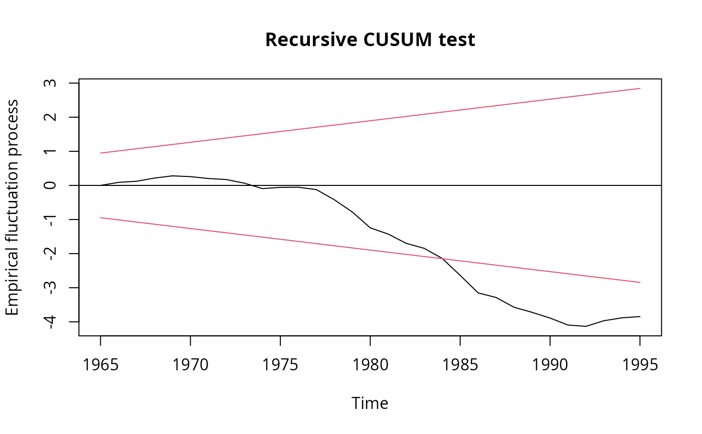 sctest(rcus)
#>
#> Recursive CUSUM test
#>
#> data: rcus
#> S = 1.4977, p-value = 0.0002437
#>
## Note: Greene's remark that the break is in 1984 (where the process crosses its boundary)
## is wrong. The break appears to be no later than 1976.
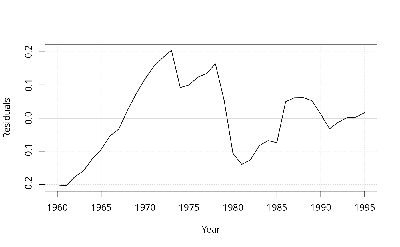
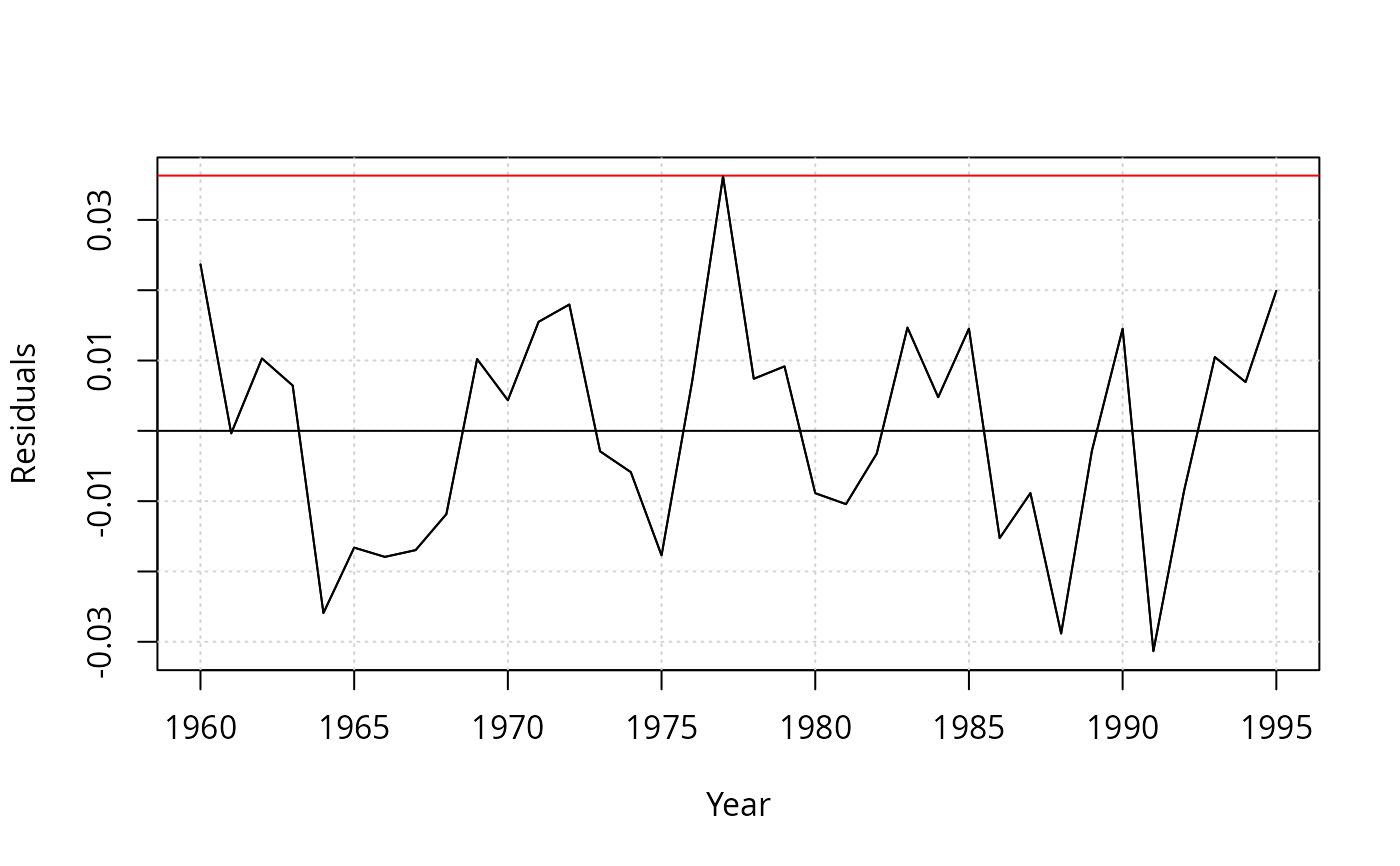
## Example 12.2
library("dynlm")
resplot <- function(obj, bound = TRUE) {
res <- residuals(obj)
sigma <- summary(obj)$sigma
plot(res, ylab = "Residuals", xlab = "Year")
grid()
abline(h = 0)
if(bound) abline(h = c(-2, 2) * sigma, col = "red")
lines(res)
}
resplot(dynlm(log(gas/population) ~ log(price), data = USGasG))
sctest(rcus)
#>
#> Recursive CUSUM test
#>
#> data: rcus
#> S = 1.4977, p-value = 0.0002437
#>
## Note: Greene's remark that the break is in 1984 (where the process crosses its boundary)
## is wrong. The break appears to be no later than 1976.
## Example 12.2
library("dynlm")
resplot <- function(obj, bound = TRUE) {
res <- residuals(obj)
sigma <- summary(obj)$sigma
plot(res, ylab = "Residuals", xlab = "Year")
grid()
abline(h = 0)
if(bound) abline(h = c(-2, 2) * sigma, col = "red")
lines(res)
}
resplot(dynlm(log(gas/population) ~ log(price), data = USGasG))
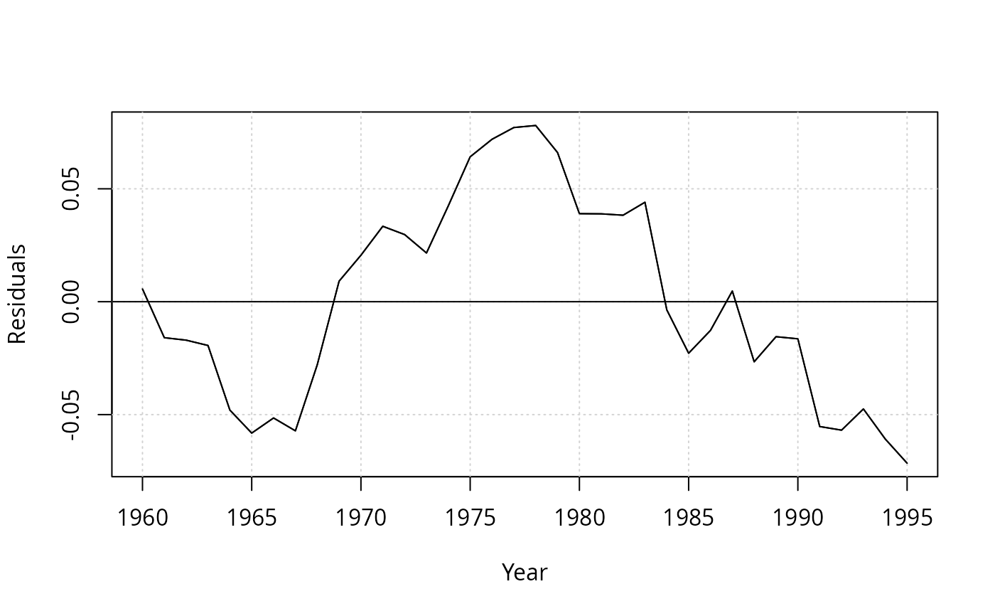
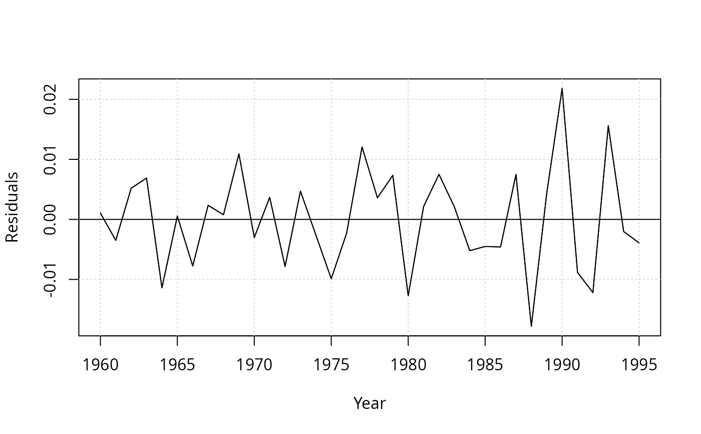
 resplot(dynlm(log(gas/population) ~ log(price) + log(income), data = USGasG))
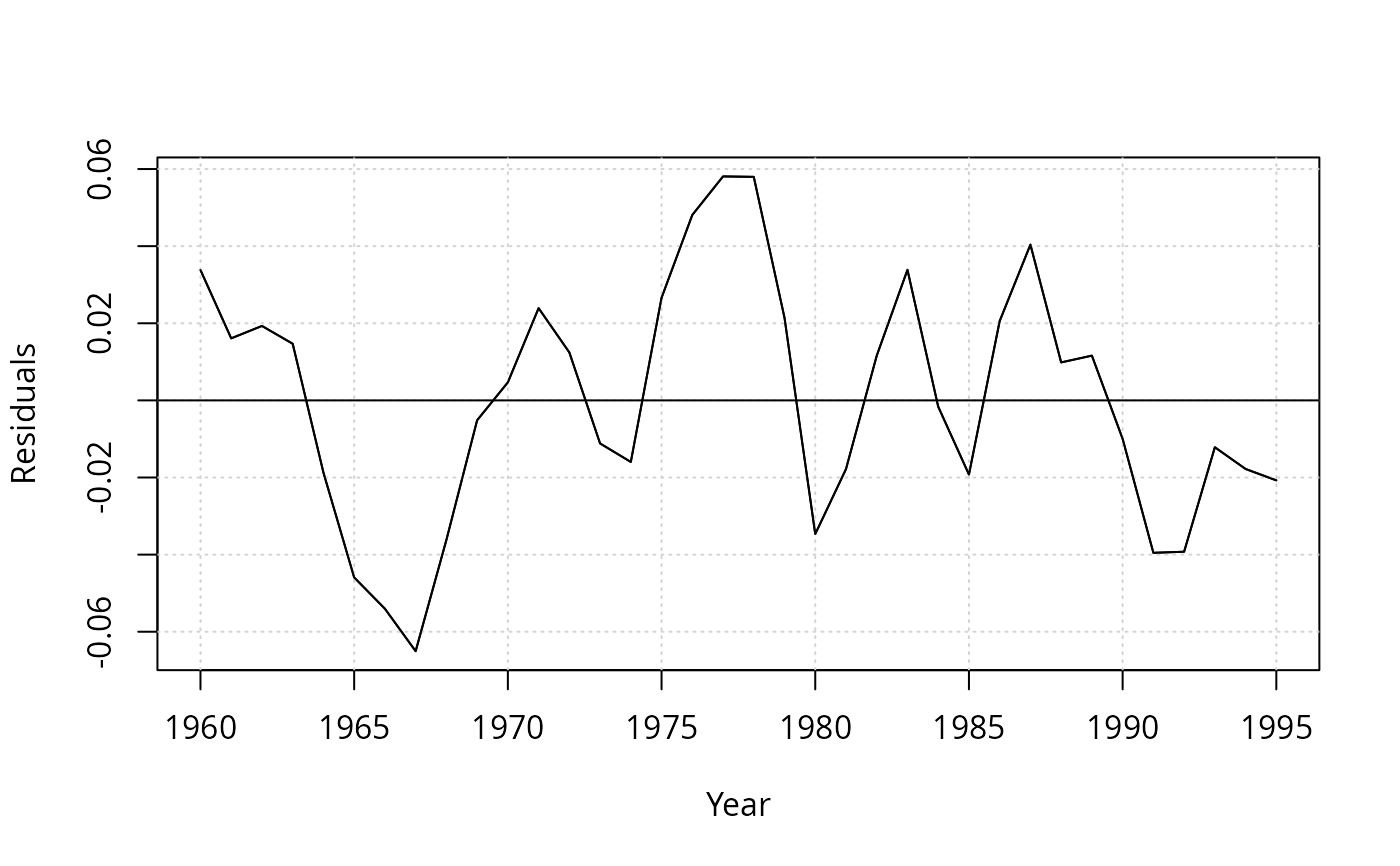
 resplot(dynlm(log(gas/population) ~ log(price) + log(income) + log(newcar) + log(usedcar) +
log(transport) + log(nondurable) + log(durable) +log(service) + ltrend, data = USGasG))
resplot(dynlm(log(gas/population) ~ log(price) + log(income) + log(newcar) + log(usedcar) +
log(transport) + log(nondurable) + log(durable) +log(service) + ltrend, data = USGasG))
 ## different shock variable than in 7.6
shock <- factor(time(USGasG) > 1974, levels = c(FALSE, TRUE), labels = c("before", "after"))
resplot(dynlm(log(gas/population) ~ shock/(log(price) + log(income) + log(newcar) + log(usedcar) +
log(transport) + log(nondurable) + log(durable) + log(service) + ltrend), data = USGasG))
## different shock variable than in 7.6
shock <- factor(time(USGasG) > 1974, levels = c(FALSE, TRUE), labels = c("before", "after"))
resplot(dynlm(log(gas/population) ~ shock/(log(price) + log(income) + log(newcar) + log(usedcar) +
log(transport) + log(nondurable) + log(durable) + log(service) + ltrend), data = USGasG))
 ## NOTE: something seems to be wrong with the sigma estimates in the `full' models
## Table 12.4, OLS
fm <- dynlm(log(gas/population) ~ log(price) + log(income) + log(newcar) + log(usedcar),
data = USGasG)
summary(fm)
#>
#> Time series regression with "ts" data:
#> Start = 1960, End = 1995
#>
#> Call:
#> dynlm(formula = log(gas/population) ~ log(price) + log(income) +
#> log(newcar) + log(usedcar), data = USGasG)
#>
#> Residuals:
#> Min 1Q Median 3Q Max
#> -0.065042 -0.018842 0.001528 0.020786 0.058084
#>
#> Coefficients:
#> Estimate Std. Error t value Pr(>|t|)
#> (Intercept) -12.34184 0.67489 -18.287 <2e-16 ***
#> log(price) -0.05910 0.03248 -1.819 0.0786 .
#> log(income) 1.37340 0.07563 18.160 <2e-16 ***
#> log(newcar) -0.12680 0.12699 -0.998 0.3258
#> log(usedcar) -0.11871 0.08134 -1.459 0.1545
#> ---
#> Signif. codes: 0 ‘***’ 0.001 ‘**’ 0.01 ‘*’ 0.05 ‘.’ 0.1 ‘ ’ 1
#>
#> Residual standard error: 0.03304 on 31 degrees of freedom
#> Multiple R-squared: 0.958, Adjusted R-squared: 0.9526
#> F-statistic: 176.7 on 4 and 31 DF, p-value: < 2.2e-16
#>
resplot(fm, bound = FALSE)
## NOTE: something seems to be wrong with the sigma estimates in the `full' models
## Table 12.4, OLS
fm <- dynlm(log(gas/population) ~ log(price) + log(income) + log(newcar) + log(usedcar),
data = USGasG)
summary(fm)
#>
#> Time series regression with "ts" data:
#> Start = 1960, End = 1995
#>
#> Call:
#> dynlm(formula = log(gas/population) ~ log(price) + log(income) +
#> log(newcar) + log(usedcar), data = USGasG)
#>
#> Residuals:
#> Min 1Q Median 3Q Max
#> -0.065042 -0.018842 0.001528 0.020786 0.058084
#>
#> Coefficients:
#> Estimate Std. Error t value Pr(>|t|)
#> (Intercept) -12.34184 0.67489 -18.287 <2e-16 ***
#> log(price) -0.05910 0.03248 -1.819 0.0786 .
#> log(income) 1.37340 0.07563 18.160 <2e-16 ***
#> log(newcar) -0.12680 0.12699 -0.998 0.3258
#> log(usedcar) -0.11871 0.08134 -1.459 0.1545
#> ---
#> Signif. codes: 0 ‘***’ 0.001 ‘**’ 0.01 ‘*’ 0.05 ‘.’ 0.1 ‘ ’ 1
#>
#> Residual standard error: 0.03304 on 31 degrees of freedom
#> Multiple R-squared: 0.958, Adjusted R-squared: 0.9526
#> F-statistic: 176.7 on 4 and 31 DF, p-value: < 2.2e-16
#>
resplot(fm, bound = FALSE)
 dwtest(fm)
#>
#> Durbin-Watson test
#>
#> data: fm
#> DW = 0.6047, p-value = 3.387e-09
#> alternative hypothesis: true autocorrelation is greater than 0
#>
## ML
g <- as.data.frame(USGasG)
y <- log(g$gas/g$population)
X <- as.matrix(cbind(log(g$price), log(g$income), log(g$newcar), log(g$usedcar)))
arima(y, order = c(1, 0, 0), xreg = X)
#>
#> Call:
#> arima(x = y, order = c(1, 0, 0), xreg = X)
#>
#> Coefficients:
#> ar1 intercept X1 X2 X3 X4
#> 0.9304 -9.7548 -0.2082 1.0818 0.0884 -0.0350
#> s.e. 0.0554 1.1262 0.0337 0.1269 0.1186 0.0612
#>
#> sigma^2 estimated as 0.0003094: log likelihood = 93.37, aic = -172.74
#######################################
## US macroeconomic data (1950-2000) ##
#######################################
## data and trend
data("USMacroG", package = "AER")
ltrend <- 0:(nrow(USMacroG) - 1)
## Example 5.3
## OLS and IV regression
library("dynlm")
fm_ols <- dynlm(consumption ~ gdp, data = USMacroG)
fm_iv <- dynlm(consumption ~ gdp | L(consumption) + L(gdp), data = USMacroG)
## Hausman statistic
library("MASS")
b_diff <- coef(fm_iv) - coef(fm_ols)
v_diff <- summary(fm_iv)$cov.unscaled - summary(fm_ols)$cov.unscaled
(t(b_diff) %*% ginv(v_diff) %*% b_diff) / summary(fm_ols)$sigma^2
#> [,1]
#> [1,] 9.703933
## Wu statistic
auxreg <- dynlm(gdp ~ L(consumption) + L(gdp), data = USMacroG)
coeftest(dynlm(consumption ~ gdp + fitted(auxreg), data = USMacroG))[3,3]
#> [1] 4.944502
## agrees with Greene (but not with errata)
## Example 6.1
## Table 6.1
fm6.1 <- dynlm(log(invest) ~ tbill + inflation + log(gdp) + ltrend, data = USMacroG)
fm6.3 <- dynlm(log(invest) ~ I(tbill - inflation) + log(gdp) + ltrend, data = USMacroG)
summary(fm6.1)
#>
#> Time series regression with "ts" data:
#> Start = 1950(2), End = 2000(4)
#>
#> Call:
#> dynlm(formula = log(invest) ~ tbill + inflation + log(gdp) +
#> ltrend, data = USMacroG)
#>
#> Residuals:
#> Min 1Q Median 3Q Max
#> -0.22313 -0.05540 -0.00312 0.04246 0.31989
#>
#> Coefficients:
#> Estimate Std. Error t value Pr(>|t|)
#> (Intercept) -9.134091 1.366459 -6.684 2.3e-10 ***
#> tbill -0.008598 0.003195 -2.691 0.00774 **
#> inflation 0.003306 0.002337 1.415 0.15872
#> log(gdp) 1.930156 0.183272 10.532 < 2e-16 ***
#> ltrend -0.005659 0.001488 -3.803 0.00019 ***
#> ---
#> Signif. codes: 0 ‘***’ 0.001 ‘**’ 0.01 ‘*’ 0.05 ‘.’ 0.1 ‘ ’ 1
#>
#> Residual standard error: 0.08618 on 198 degrees of freedom
#> (1 observation deleted due to missingness)
#> Multiple R-squared: 0.9798, Adjusted R-squared: 0.9793
#> F-statistic: 2395 on 4 and 198 DF, p-value: < 2.2e-16
#>
summary(fm6.3)
#>
#> Time series regression with "ts" data:
#> Start = 1950(2), End = 2000(4)
#>
#> Call:
#> dynlm(formula = log(invest) ~ I(tbill - inflation) + log(gdp) +
#> ltrend, data = USMacroG)
#>
#> Residuals:
#> Min 1Q Median 3Q Max
#> -0.227897 -0.054542 -0.002435 0.039993 0.313928
#>
#> Coefficients:
#> Estimate Std. Error t value Pr(>|t|)
#> (Intercept) -7.907158 1.200631 -6.586 3.94e-10 ***
#> I(tbill - inflation) -0.004427 0.002270 -1.950 0.05260 .
#> log(gdp) 1.764062 0.160561 10.987 < 2e-16 ***
#> ltrend -0.004403 0.001331 -3.308 0.00111 **
#> ---
#> Signif. codes: 0 ‘***’ 0.001 ‘**’ 0.01 ‘*’ 0.05 ‘.’ 0.1 ‘ ’ 1
#>
#> Residual standard error: 0.0867 on 199 degrees of freedom
#> (1 observation deleted due to missingness)
#> Multiple R-squared: 0.9794, Adjusted R-squared: 0.9791
#> F-statistic: 3154 on 3 and 199 DF, p-value: < 2.2e-16
#>
deviance(fm6.1)
#> [1] 1.470565
deviance(fm6.3)
#> [1] 1.495811
vcov(fm6.1)[2,3]
#> [1] -3.717454e-06
## F test
linearHypothesis(fm6.1, "tbill + inflation = 0")
#>
#> Linear hypothesis test:
#> tbill + inflation = 0
#>
#> Model 1: restricted model
#> Model 2: log(invest) ~ tbill + inflation + log(gdp) + ltrend
#>
#> Res.Df RSS Df Sum of Sq F Pr(>F)
#> 1 199 1.4958
#> 2 198 1.4706 1 0.025246 3.3991 0.06673 .
#> ---
#> Signif. codes: 0 ‘***’ 0.001 ‘**’ 0.01 ‘*’ 0.05 ‘.’ 0.1 ‘ ’ 1
## alternatively
anova(fm6.1, fm6.3)
#> Analysis of Variance Table
#>
#> Model 1: log(invest) ~ tbill + inflation + log(gdp) + ltrend
#> Model 2: log(invest) ~ I(tbill - inflation) + log(gdp) + ltrend
#> Res.Df RSS Df Sum of Sq F Pr(>F)
#> 1 198 1.4706
#> 2 199 1.4958 -1 -0.025246 3.3991 0.06673 .
#> ---
#> Signif. codes: 0 ‘***’ 0.001 ‘**’ 0.01 ‘*’ 0.05 ‘.’ 0.1 ‘ ’ 1
## t statistic
sqrt(anova(fm6.1, fm6.3)[2,5])
#> [1] 1.843672
## Example 6.3
## Distributed lag model:
## log(Ct) = b0 + b1 * log(Yt) + b2 * log(C(t-1)) + u
us <- log(USMacroG[, c(2, 5)])
fm_distlag <- dynlm(log(consumption) ~ log(dpi) + L(log(consumption)),
data = USMacroG)
summary(fm_distlag)
#>
#> Time series regression with "ts" data:
#> Start = 1950(2), End = 2000(4)
#>
#> Call:
#> dynlm(formula = log(consumption) ~ log(dpi) + L(log(consumption)),
#> data = USMacroG)
#>
#> Residuals:
#> Min 1Q Median 3Q Max
#> -0.035243 -0.004606 0.000496 0.005147 0.041754
#>
#> Coefficients:
#> Estimate Std. Error t value Pr(>|t|)
#> (Intercept) 0.003142 0.010553 0.298 0.76624
#> log(dpi) 0.074958 0.028727 2.609 0.00976 **
#> L(log(consumption)) 0.924625 0.028594 32.337 < 2e-16 ***
#> ---
#> Signif. codes: 0 ‘***’ 0.001 ‘**’ 0.01 ‘*’ 0.05 ‘.’ 0.1 ‘ ’ 1
#>
#> Residual standard error: 0.008742 on 200 degrees of freedom
#> Multiple R-squared: 0.9997, Adjusted R-squared: 0.9997
#> F-statistic: 3.476e+05 on 2 and 200 DF, p-value: < 2.2e-16
#>
## estimate and test long-run MPC
coef(fm_distlag)[2]/(1-coef(fm_distlag)[3])
#> log(dpi)
#> 0.9944606
linearHypothesis(fm_distlag, "log(dpi) + L(log(consumption)) = 1")
#>
#> Linear hypothesis test:
#> log(dpi) + L(log(consumption)) = 1
#>
#> Model 1: restricted model
#> Model 2: log(consumption) ~ log(dpi) + L(log(consumption))
#>
#> Res.Df RSS Df Sum of Sq F Pr(>F)
#> 1 201 0.015295
#> 2 200 0.015286 1 9.1197e-06 0.1193 0.7301
## correct, see errata
## Example 6.4
## predict investiment in 2001(1)
predict(fm6.1, interval = "prediction",
newdata = data.frame(tbill = 4.48, inflation = 5.262, gdp = 9316.8, ltrend = 204))
#> fit lwr upr
#> 1 7.331178 7.158229 7.504126
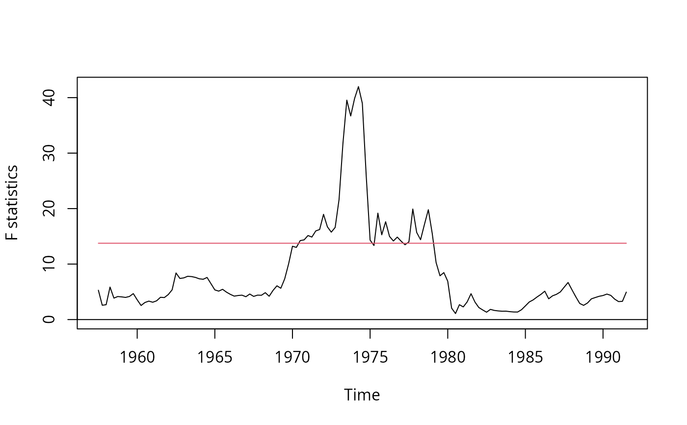
## Example 7.7
## no GMM available in "strucchange"
## using OLS instead yields
fs <- Fstats(log(m1/cpi) ~ log(gdp) + tbill, data = USMacroG,
vcov = NeweyWest, from = c(1957, 3), to = c(1991, 3))
plot(fs)
dwtest(fm)
#>
#> Durbin-Watson test
#>
#> data: fm
#> DW = 0.6047, p-value = 3.387e-09
#> alternative hypothesis: true autocorrelation is greater than 0
#>
## ML
g <- as.data.frame(USGasG)
y <- log(g$gas/g$population)
X <- as.matrix(cbind(log(g$price), log(g$income), log(g$newcar), log(g$usedcar)))
arima(y, order = c(1, 0, 0), xreg = X)
#>
#> Call:
#> arima(x = y, order = c(1, 0, 0), xreg = X)
#>
#> Coefficients:
#> ar1 intercept X1 X2 X3 X4
#> 0.9304 -9.7548 -0.2082 1.0818 0.0884 -0.0350
#> s.e. 0.0554 1.1262 0.0337 0.1269 0.1186 0.0612
#>
#> sigma^2 estimated as 0.0003094: log likelihood = 93.37, aic = -172.74
#######################################
## US macroeconomic data (1950-2000) ##
#######################################
## data and trend
data("USMacroG", package = "AER")
ltrend <- 0:(nrow(USMacroG) - 1)
## Example 5.3
## OLS and IV regression
library("dynlm")
fm_ols <- dynlm(consumption ~ gdp, data = USMacroG)
fm_iv <- dynlm(consumption ~ gdp | L(consumption) + L(gdp), data = USMacroG)
## Hausman statistic
library("MASS")
b_diff <- coef(fm_iv) - coef(fm_ols)
v_diff <- summary(fm_iv)$cov.unscaled - summary(fm_ols)$cov.unscaled
(t(b_diff) %*% ginv(v_diff) %*% b_diff) / summary(fm_ols)$sigma^2
#> [,1]
#> [1,] 9.703933
## Wu statistic
auxreg <- dynlm(gdp ~ L(consumption) + L(gdp), data = USMacroG)
coeftest(dynlm(consumption ~ gdp + fitted(auxreg), data = USMacroG))[3,3]
#> [1] 4.944502
## agrees with Greene (but not with errata)
## Example 6.1
## Table 6.1
fm6.1 <- dynlm(log(invest) ~ tbill + inflation + log(gdp) + ltrend, data = USMacroG)
fm6.3 <- dynlm(log(invest) ~ I(tbill - inflation) + log(gdp) + ltrend, data = USMacroG)
summary(fm6.1)
#>
#> Time series regression with "ts" data:
#> Start = 1950(2), End = 2000(4)
#>
#> Call:
#> dynlm(formula = log(invest) ~ tbill + inflation + log(gdp) +
#> ltrend, data = USMacroG)
#>
#> Residuals:
#> Min 1Q Median 3Q Max
#> -0.22313 -0.05540 -0.00312 0.04246 0.31989
#>
#> Coefficients:
#> Estimate Std. Error t value Pr(>|t|)
#> (Intercept) -9.134091 1.366459 -6.684 2.3e-10 ***
#> tbill -0.008598 0.003195 -2.691 0.00774 **
#> inflation 0.003306 0.002337 1.415 0.15872
#> log(gdp) 1.930156 0.183272 10.532 < 2e-16 ***
#> ltrend -0.005659 0.001488 -3.803 0.00019 ***
#> ---
#> Signif. codes: 0 ‘***’ 0.001 ‘**’ 0.01 ‘*’ 0.05 ‘.’ 0.1 ‘ ’ 1
#>
#> Residual standard error: 0.08618 on 198 degrees of freedom
#> (1 observation deleted due to missingness)
#> Multiple R-squared: 0.9798, Adjusted R-squared: 0.9793
#> F-statistic: 2395 on 4 and 198 DF, p-value: < 2.2e-16
#>
summary(fm6.3)
#>
#> Time series regression with "ts" data:
#> Start = 1950(2), End = 2000(4)
#>
#> Call:
#> dynlm(formula = log(invest) ~ I(tbill - inflation) + log(gdp) +
#> ltrend, data = USMacroG)
#>
#> Residuals:
#> Min 1Q Median 3Q Max
#> -0.227897 -0.054542 -0.002435 0.039993 0.313928
#>
#> Coefficients:
#> Estimate Std. Error t value Pr(>|t|)
#> (Intercept) -7.907158 1.200631 -6.586 3.94e-10 ***
#> I(tbill - inflation) -0.004427 0.002270 -1.950 0.05260 .
#> log(gdp) 1.764062 0.160561 10.987 < 2e-16 ***
#> ltrend -0.004403 0.001331 -3.308 0.00111 **
#> ---
#> Signif. codes: 0 ‘***’ 0.001 ‘**’ 0.01 ‘*’ 0.05 ‘.’ 0.1 ‘ ’ 1
#>
#> Residual standard error: 0.0867 on 199 degrees of freedom
#> (1 observation deleted due to missingness)
#> Multiple R-squared: 0.9794, Adjusted R-squared: 0.9791
#> F-statistic: 3154 on 3 and 199 DF, p-value: < 2.2e-16
#>
deviance(fm6.1)
#> [1] 1.470565
deviance(fm6.3)
#> [1] 1.495811
vcov(fm6.1)[2,3]
#> [1] -3.717454e-06
## F test
linearHypothesis(fm6.1, "tbill + inflation = 0")
#>
#> Linear hypothesis test:
#> tbill + inflation = 0
#>
#> Model 1: restricted model
#> Model 2: log(invest) ~ tbill + inflation + log(gdp) + ltrend
#>
#> Res.Df RSS Df Sum of Sq F Pr(>F)
#> 1 199 1.4958
#> 2 198 1.4706 1 0.025246 3.3991 0.06673 .
#> ---
#> Signif. codes: 0 ‘***’ 0.001 ‘**’ 0.01 ‘*’ 0.05 ‘.’ 0.1 ‘ ’ 1
## alternatively
anova(fm6.1, fm6.3)
#> Analysis of Variance Table
#>
#> Model 1: log(invest) ~ tbill + inflation + log(gdp) + ltrend
#> Model 2: log(invest) ~ I(tbill - inflation) + log(gdp) + ltrend
#> Res.Df RSS Df Sum of Sq F Pr(>F)
#> 1 198 1.4706
#> 2 199 1.4958 -1 -0.025246 3.3991 0.06673 .
#> ---
#> Signif. codes: 0 ‘***’ 0.001 ‘**’ 0.01 ‘*’ 0.05 ‘.’ 0.1 ‘ ’ 1
## t statistic
sqrt(anova(fm6.1, fm6.3)[2,5])
#> [1] 1.843672
## Example 6.3
## Distributed lag model:
## log(Ct) = b0 + b1 * log(Yt) + b2 * log(C(t-1)) + u
us <- log(USMacroG[, c(2, 5)])
fm_distlag <- dynlm(log(consumption) ~ log(dpi) + L(log(consumption)),
data = USMacroG)
summary(fm_distlag)
#>
#> Time series regression with "ts" data:
#> Start = 1950(2), End = 2000(4)
#>
#> Call:
#> dynlm(formula = log(consumption) ~ log(dpi) + L(log(consumption)),
#> data = USMacroG)
#>
#> Residuals:
#> Min 1Q Median 3Q Max
#> -0.035243 -0.004606 0.000496 0.005147 0.041754
#>
#> Coefficients:
#> Estimate Std. Error t value Pr(>|t|)
#> (Intercept) 0.003142 0.010553 0.298 0.76624
#> log(dpi) 0.074958 0.028727 2.609 0.00976 **
#> L(log(consumption)) 0.924625 0.028594 32.337 < 2e-16 ***
#> ---
#> Signif. codes: 0 ‘***’ 0.001 ‘**’ 0.01 ‘*’ 0.05 ‘.’ 0.1 ‘ ’ 1
#>
#> Residual standard error: 0.008742 on 200 degrees of freedom
#> Multiple R-squared: 0.9997, Adjusted R-squared: 0.9997
#> F-statistic: 3.476e+05 on 2 and 200 DF, p-value: < 2.2e-16
#>
## estimate and test long-run MPC
coef(fm_distlag)[2]/(1-coef(fm_distlag)[3])
#> log(dpi)
#> 0.9944606
linearHypothesis(fm_distlag, "log(dpi) + L(log(consumption)) = 1")
#>
#> Linear hypothesis test:
#> log(dpi) + L(log(consumption)) = 1
#>
#> Model 1: restricted model
#> Model 2: log(consumption) ~ log(dpi) + L(log(consumption))
#>
#> Res.Df RSS Df Sum of Sq F Pr(>F)
#> 1 201 0.015295
#> 2 200 0.015286 1 9.1197e-06 0.1193 0.7301
## correct, see errata
## Example 6.4
## predict investiment in 2001(1)
predict(fm6.1, interval = "prediction",
newdata = data.frame(tbill = 4.48, inflation = 5.262, gdp = 9316.8, ltrend = 204))
#> fit lwr upr
#> 1 7.331178 7.158229 7.504126
## Example 7.7
## no GMM available in "strucchange"
## using OLS instead yields
fs <- Fstats(log(m1/cpi) ~ log(gdp) + tbill, data = USMacroG,
vcov = NeweyWest, from = c(1957, 3), to = c(1991, 3))
plot(fs)
 ## which looks somewhat similar ...
## Example 8.2
## Ct = b0 + b1*Yt + b2*Y(t-1) + v
fm1 <- dynlm(consumption ~ dpi + L(dpi), data = USMacroG)
## Ct = a0 + a1*Yt + a2*C(t-1) + u
fm2 <- dynlm(consumption ~ dpi + L(consumption), data = USMacroG)
## Cox test in both directions:
coxtest(fm1, fm2)
#> Cox test
#>
#> Model 1: consumption ~ dpi + L(dpi)
#> Model 2: consumption ~ dpi + L(consumption)
#> Estimate Std. Error z value Pr(>|z|)
#> fitted(M1) ~ M2 -284.908 0.01862 -15304.2817 < 2.2e-16 ***
#> fitted(M2) ~ M1 1.491 0.42735 3.4894 0.0004842 ***
#> ---
#> Signif. codes: 0 ‘***’ 0.001 ‘**’ 0.01 ‘*’ 0.05 ‘.’ 0.1 ‘ ’ 1
## ... and do the same for jtest() and encomptest().
## Notice that in this particular case two of them are coincident.
jtest(fm1, fm2)
#> J test
#>
#> Model 1: consumption ~ dpi + L(dpi)
#> Model 2: consumption ~ dpi + L(consumption)
#> Estimate Std. Error t value Pr(>|t|)
#> M1 + fitted(M2) 1.0145 0.01614 62.8605 < 2.2e-16 ***
#> M2 + fitted(M1) -10.6766 1.48542 -7.1876 1.299e-11 ***
#> ---
#> Signif. codes: 0 ‘***’ 0.001 ‘**’ 0.01 ‘*’ 0.05 ‘.’ 0.1 ‘ ’ 1
encomptest(fm1, fm2)
#> Encompassing test
#>
#> Model 1: consumption ~ dpi + L(dpi)
#> Model 2: consumption ~ dpi + L(consumption)
#> Model E: consumption ~ dpi + L(dpi) + L(consumption)
#> Res.Df Df F Pr(>F)
#> M1 vs. ME 199 -1 3951.448 < 2.2e-16 ***
#> M2 vs. ME 199 -1 51.661 1.299e-11 ***
#> ---
#> Signif. codes: 0 ‘***’ 0.001 ‘**’ 0.01 ‘*’ 0.05 ‘.’ 0.1 ‘ ’ 1
## encomptest could also be performed `by hand' via
fmE <- dynlm(consumption ~ dpi + L(dpi) + L(consumption), data = USMacroG)
waldtest(fm1, fmE, fm2)
#> Wald test
#>
#> Model 1: consumption ~ dpi + L(dpi)
#> Model 2: consumption ~ dpi + L(dpi) + L(consumption)
#> Model 3: consumption ~ dpi + L(consumption)
#> Res.Df Df F Pr(>F)
#> 1 200
#> 2 199 1 3951.448 < 2.2e-16 ***
#> 3 200 -1 51.661 1.299e-11 ***
#> ---
#> Signif. codes: 0 ‘***’ 0.001 ‘**’ 0.01 ‘*’ 0.05 ‘.’ 0.1 ‘ ’ 1
## Table 9.1
fm_ols <- lm(consumption ~ dpi, data = as.data.frame(USMacroG))
fm_nls <- nls(consumption ~ alpha + beta * dpi^gamma,
start = list(alpha = coef(fm_ols)[1], beta = coef(fm_ols)[2], gamma = 1),
control = nls.control(maxiter = 100), data = as.data.frame(USMacroG))
summary(fm_ols)
#>
#> Call:
#> lm(formula = consumption ~ dpi, data = as.data.frame(USMacroG))
#>
#> Residuals:
#> Min 1Q Median 3Q Max
#> -191.42 -56.08 1.38 49.53 324.14
#>
#> Coefficients:
#> Estimate Std. Error t value Pr(>|t|)
#> (Intercept) -80.354749 14.305852 -5.617 6.38e-08 ***
#> dpi 0.921686 0.003872 238.054 < 2e-16 ***
#> ---
#> Signif. codes: 0 ‘***’ 0.001 ‘**’ 0.01 ‘*’ 0.05 ‘.’ 0.1 ‘ ’ 1
#>
#> Residual standard error: 87.21 on 202 degrees of freedom
#> Multiple R-squared: 0.9964, Adjusted R-squared: 0.9964
#> F-statistic: 5.667e+04 on 1 and 202 DF, p-value: < 2.2e-16
#>
summary(fm_nls)
#>
#> Formula: consumption ~ alpha + beta * dpi^gamma
#>
#> Parameters:
#> Estimate Std. Error t value Pr(>|t|)
#> alpha 458.79850 22.50142 20.390 <2e-16 ***
#> beta 0.10085 0.01091 9.244 <2e-16 ***
#> gamma 1.24483 0.01205 103.263 <2e-16 ***
#> ---
#> Signif. codes: 0 ‘***’ 0.001 ‘**’ 0.01 ‘*’ 0.05 ‘.’ 0.1 ‘ ’ 1
#>
#> Residual standard error: 50.09 on 201 degrees of freedom
#>
#> Number of iterations to convergence: 64
#> Achieved convergence tolerance: 1.701e-06
#>
deviance(fm_ols)
#> [1] 1536322
deviance(fm_nls)
#> [1] 504403.2
vcov(fm_nls)
#> alpha beta gamma
#> alpha 506.3137170 -0.2345464898 0.2575688410
#> beta -0.2345465 0.0001190378 -0.0001314916
#> gamma 0.2575688 -0.0001314916 0.0001453206
## Example 9.7
## F test
fm_nls2 <- nls(consumption ~ alpha + beta * dpi,
start = list(alpha = coef(fm_ols)[1], beta = coef(fm_ols)[2]),
control = nls.control(maxiter = 100), data = as.data.frame(USMacroG))
anova(fm_nls, fm_nls2)
#> Analysis of Variance Table
#>
#> Model 1: consumption ~ alpha + beta * dpi^gamma
#> Model 2: consumption ~ alpha + beta * dpi
#> Res.Df Res.Sum Sq Df Sum Sq F value Pr(>F)
#> 1 201 504403
#> 2 202 1536322 -1 -1031919 411.21 < 2.2e-16 ***
#> ---
#> Signif. codes: 0 ‘***’ 0.001 ‘**’ 0.01 ‘*’ 0.05 ‘.’ 0.1 ‘ ’ 1
## Wald test
linearHypothesis(fm_nls, "gamma = 1")
#>
#> Linear hypothesis test:
#> gamma = 1
#>
#> Model 1: restricted model
#> Model 2: consumption ~ alpha + beta * dpi^gamma
#>
#> Res.Df Df Chisq Pr(>Chisq)
#> 1 202
#> 2 201 1 412.47 < 2.2e-16 ***
#> ---
#> Signif. codes: 0 ‘***’ 0.001 ‘**’ 0.01 ‘*’ 0.05 ‘.’ 0.1 ‘ ’ 1
## Example 9.8, Table 9.2
usm <- USMacroG[, c("m1", "tbill", "gdp")]
fm_lin <- lm(m1 ~ tbill + gdp, data = usm)
fm_log <- lm(m1 ~ tbill + gdp, data = log(usm))
## PE auxiliary regressions
aux_lin <- lm(m1 ~ tbill + gdp + I(fitted(fm_log) - log(fitted(fm_lin))), data = usm)
aux_log <- lm(m1 ~ tbill + gdp + I(fitted(fm_lin) - exp(fitted(fm_log))), data = log(usm))
coeftest(aux_lin)[4,]
#> Estimate Std. Error t value Pr(>|t|)
#> 2.093544e+02 2.675803e+01 7.823985e+00 2.900156e-13
coeftest(aux_log)[4,]
#> Estimate Std. Error t value Pr(>|t|)
#> -4.188803e-05 2.613270e-04 -1.602897e-01 8.728146e-01
## matches results from errata
## With lmtest >= 0.9-24:
## petest(fm_lin, fm_log)
## Example 12.1
fm_m1 <- dynlm(log(m1) ~ log(gdp) + log(cpi), data = USMacroG)
summary(fm_m1)
#>
#> Time series regression with "ts" data:
#> Start = 1950(1), End = 2000(4)
#>
#> Call:
#> dynlm(formula = log(m1) ~ log(gdp) + log(cpi), data = USMacroG)
#>
#> Residuals:
#> Min 1Q Median 3Q Max
#> -0.230620 -0.026026 0.008483 0.036407 0.205929
#>
#> Coefficients:
#> Estimate Std. Error t value Pr(>|t|)
#> (Intercept) -1.63306 0.22857 -7.145 1.62e-11 ***
#> log(gdp) 0.28705 0.04738 6.058 6.68e-09 ***
#> log(cpi) 0.97181 0.03377 28.775 < 2e-16 ***
#> ---
#> Signif. codes: 0 ‘***’ 0.001 ‘**’ 0.01 ‘*’ 0.05 ‘.’ 0.1 ‘ ’ 1
#>
#> Residual standard error: 0.08288 on 201 degrees of freedom
#> Multiple R-squared: 0.9895, Adjusted R-squared: 0.9894
#> F-statistic: 9489 on 2 and 201 DF, p-value: < 2.2e-16
#>
## Figure 12.1
par(las = 1)
plot(0, 0, type = "n", axes = FALSE,
xlim = c(1950, 2002), ylim = c(-0.3, 0.225),
xaxs = "i", yaxs = "i",
xlab = "Quarter", ylab = "", main = "Least Squares Residuals")
box()
axis(1, at = c(1950, 1963, 1976, 1989, 2002))
axis(2, seq(-0.3, 0.225, by = 0.075))
grid(4, 7, col = grey(0.6))
abline(0, 0)
lines(residuals(fm_m1), lwd = 2)
## which looks somewhat similar ...
## Example 8.2
## Ct = b0 + b1*Yt + b2*Y(t-1) + v
fm1 <- dynlm(consumption ~ dpi + L(dpi), data = USMacroG)
## Ct = a0 + a1*Yt + a2*C(t-1) + u
fm2 <- dynlm(consumption ~ dpi + L(consumption), data = USMacroG)
## Cox test in both directions:
coxtest(fm1, fm2)
#> Cox test
#>
#> Model 1: consumption ~ dpi + L(dpi)
#> Model 2: consumption ~ dpi + L(consumption)
#> Estimate Std. Error z value Pr(>|z|)
#> fitted(M1) ~ M2 -284.908 0.01862 -15304.2817 < 2.2e-16 ***
#> fitted(M2) ~ M1 1.491 0.42735 3.4894 0.0004842 ***
#> ---
#> Signif. codes: 0 ‘***’ 0.001 ‘**’ 0.01 ‘*’ 0.05 ‘.’ 0.1 ‘ ’ 1
## ... and do the same for jtest() and encomptest().
## Notice that in this particular case two of them are coincident.
jtest(fm1, fm2)
#> J test
#>
#> Model 1: consumption ~ dpi + L(dpi)
#> Model 2: consumption ~ dpi + L(consumption)
#> Estimate Std. Error t value Pr(>|t|)
#> M1 + fitted(M2) 1.0145 0.01614 62.8605 < 2.2e-16 ***
#> M2 + fitted(M1) -10.6766 1.48542 -7.1876 1.299e-11 ***
#> ---
#> Signif. codes: 0 ‘***’ 0.001 ‘**’ 0.01 ‘*’ 0.05 ‘.’ 0.1 ‘ ’ 1
encomptest(fm1, fm2)
#> Encompassing test
#>
#> Model 1: consumption ~ dpi + L(dpi)
#> Model 2: consumption ~ dpi + L(consumption)
#> Model E: consumption ~ dpi + L(dpi) + L(consumption)
#> Res.Df Df F Pr(>F)
#> M1 vs. ME 199 -1 3951.448 < 2.2e-16 ***
#> M2 vs. ME 199 -1 51.661 1.299e-11 ***
#> ---
#> Signif. codes: 0 ‘***’ 0.001 ‘**’ 0.01 ‘*’ 0.05 ‘.’ 0.1 ‘ ’ 1
## encomptest could also be performed `by hand' via
fmE <- dynlm(consumption ~ dpi + L(dpi) + L(consumption), data = USMacroG)
waldtest(fm1, fmE, fm2)
#> Wald test
#>
#> Model 1: consumption ~ dpi + L(dpi)
#> Model 2: consumption ~ dpi + L(dpi) + L(consumption)
#> Model 3: consumption ~ dpi + L(consumption)
#> Res.Df Df F Pr(>F)
#> 1 200
#> 2 199 1 3951.448 < 2.2e-16 ***
#> 3 200 -1 51.661 1.299e-11 ***
#> ---
#> Signif. codes: 0 ‘***’ 0.001 ‘**’ 0.01 ‘*’ 0.05 ‘.’ 0.1 ‘ ’ 1
## Table 9.1
fm_ols <- lm(consumption ~ dpi, data = as.data.frame(USMacroG))
fm_nls <- nls(consumption ~ alpha + beta * dpi^gamma,
start = list(alpha = coef(fm_ols)[1], beta = coef(fm_ols)[2], gamma = 1),
control = nls.control(maxiter = 100), data = as.data.frame(USMacroG))
summary(fm_ols)
#>
#> Call:
#> lm(formula = consumption ~ dpi, data = as.data.frame(USMacroG))
#>
#> Residuals:
#> Min 1Q Median 3Q Max
#> -191.42 -56.08 1.38 49.53 324.14
#>
#> Coefficients:
#> Estimate Std. Error t value Pr(>|t|)
#> (Intercept) -80.354749 14.305852 -5.617 6.38e-08 ***
#> dpi 0.921686 0.003872 238.054 < 2e-16 ***
#> ---
#> Signif. codes: 0 ‘***’ 0.001 ‘**’ 0.01 ‘*’ 0.05 ‘.’ 0.1 ‘ ’ 1
#>
#> Residual standard error: 87.21 on 202 degrees of freedom
#> Multiple R-squared: 0.9964, Adjusted R-squared: 0.9964
#> F-statistic: 5.667e+04 on 1 and 202 DF, p-value: < 2.2e-16
#>
summary(fm_nls)
#>
#> Formula: consumption ~ alpha + beta * dpi^gamma
#>
#> Parameters:
#> Estimate Std. Error t value Pr(>|t|)
#> alpha 458.79850 22.50142 20.390 <2e-16 ***
#> beta 0.10085 0.01091 9.244 <2e-16 ***
#> gamma 1.24483 0.01205 103.263 <2e-16 ***
#> ---
#> Signif. codes: 0 ‘***’ 0.001 ‘**’ 0.01 ‘*’ 0.05 ‘.’ 0.1 ‘ ’ 1
#>
#> Residual standard error: 50.09 on 201 degrees of freedom
#>
#> Number of iterations to convergence: 64
#> Achieved convergence tolerance: 1.701e-06
#>
deviance(fm_ols)
#> [1] 1536322
deviance(fm_nls)
#> [1] 504403.2
vcov(fm_nls)
#> alpha beta gamma
#> alpha 506.3137170 -0.2345464898 0.2575688410
#> beta -0.2345465 0.0001190378 -0.0001314916
#> gamma 0.2575688 -0.0001314916 0.0001453206
## Example 9.7
## F test
fm_nls2 <- nls(consumption ~ alpha + beta * dpi,
start = list(alpha = coef(fm_ols)[1], beta = coef(fm_ols)[2]),
control = nls.control(maxiter = 100), data = as.data.frame(USMacroG))
anova(fm_nls, fm_nls2)
#> Analysis of Variance Table
#>
#> Model 1: consumption ~ alpha + beta * dpi^gamma
#> Model 2: consumption ~ alpha + beta * dpi
#> Res.Df Res.Sum Sq Df Sum Sq F value Pr(>F)
#> 1 201 504403
#> 2 202 1536322 -1 -1031919 411.21 < 2.2e-16 ***
#> ---
#> Signif. codes: 0 ‘***’ 0.001 ‘**’ 0.01 ‘*’ 0.05 ‘.’ 0.1 ‘ ’ 1
## Wald test
linearHypothesis(fm_nls, "gamma = 1")
#>
#> Linear hypothesis test:
#> gamma = 1
#>
#> Model 1: restricted model
#> Model 2: consumption ~ alpha + beta * dpi^gamma
#>
#> Res.Df Df Chisq Pr(>Chisq)
#> 1 202
#> 2 201 1 412.47 < 2.2e-16 ***
#> ---
#> Signif. codes: 0 ‘***’ 0.001 ‘**’ 0.01 ‘*’ 0.05 ‘.’ 0.1 ‘ ’ 1
## Example 9.8, Table 9.2
usm <- USMacroG[, c("m1", "tbill", "gdp")]
fm_lin <- lm(m1 ~ tbill + gdp, data = usm)
fm_log <- lm(m1 ~ tbill + gdp, data = log(usm))
## PE auxiliary regressions
aux_lin <- lm(m1 ~ tbill + gdp + I(fitted(fm_log) - log(fitted(fm_lin))), data = usm)
aux_log <- lm(m1 ~ tbill + gdp + I(fitted(fm_lin) - exp(fitted(fm_log))), data = log(usm))
coeftest(aux_lin)[4,]
#> Estimate Std. Error t value Pr(>|t|)
#> 2.093544e+02 2.675803e+01 7.823985e+00 2.900156e-13
coeftest(aux_log)[4,]
#> Estimate Std. Error t value Pr(>|t|)
#> -4.188803e-05 2.613270e-04 -1.602897e-01 8.728146e-01
## matches results from errata
## With lmtest >= 0.9-24:
## petest(fm_lin, fm_log)
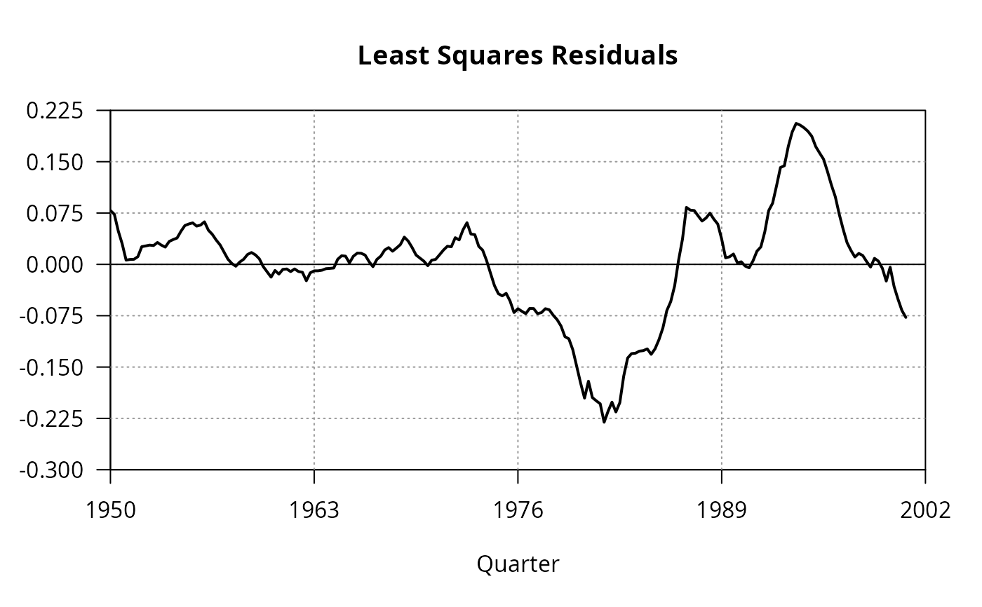
## Example 12.1
fm_m1 <- dynlm(log(m1) ~ log(gdp) + log(cpi), data = USMacroG)
summary(fm_m1)
#>
#> Time series regression with "ts" data:
#> Start = 1950(1), End = 2000(4)
#>
#> Call:
#> dynlm(formula = log(m1) ~ log(gdp) + log(cpi), data = USMacroG)
#>
#> Residuals:
#> Min 1Q Median 3Q Max
#> -0.230620 -0.026026 0.008483 0.036407 0.205929
#>
#> Coefficients:
#> Estimate Std. Error t value Pr(>|t|)
#> (Intercept) -1.63306 0.22857 -7.145 1.62e-11 ***
#> log(gdp) 0.28705 0.04738 6.058 6.68e-09 ***
#> log(cpi) 0.97181 0.03377 28.775 < 2e-16 ***
#> ---
#> Signif. codes: 0 ‘***’ 0.001 ‘**’ 0.01 ‘*’ 0.05 ‘.’ 0.1 ‘ ’ 1
#>
#> Residual standard error: 0.08288 on 201 degrees of freedom
#> Multiple R-squared: 0.9895, Adjusted R-squared: 0.9894
#> F-statistic: 9489 on 2 and 201 DF, p-value: < 2.2e-16
#>
## Figure 12.1
par(las = 1)
plot(0, 0, type = "n", axes = FALSE,
xlim = c(1950, 2002), ylim = c(-0.3, 0.225),
xaxs = "i", yaxs = "i",
xlab = "Quarter", ylab = "", main = "Least Squares Residuals")
box()
axis(1, at = c(1950, 1963, 1976, 1989, 2002))
axis(2, seq(-0.3, 0.225, by = 0.075))
grid(4, 7, col = grey(0.6))
abline(0, 0)
lines(residuals(fm_m1), lwd = 2)
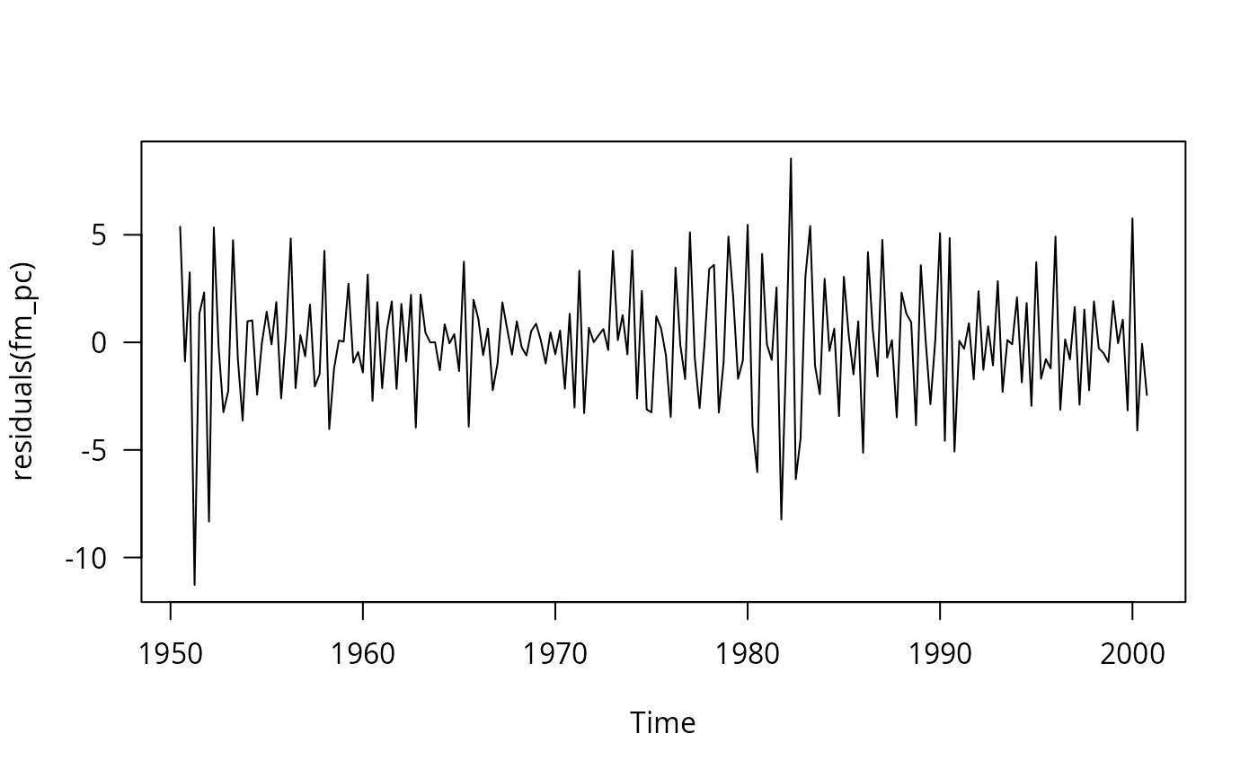
 ## Example 12.3
fm_pc <- dynlm(d(inflation) ~ unemp, data = USMacroG)
summary(fm_pc)
#>
#> Time series regression with "ts" data:
#> Start = 1950(3), End = 2000(4)
#>
#> Call:
#> dynlm(formula = d(inflation) ~ unemp, data = USMacroG)
#>
#> Residuals:
#> Min 1Q Median 3Q Max
#> -11.2791 -1.6635 -0.0117 1.7813 8.5472
#>
#> Coefficients:
#> Estimate Std. Error t value Pr(>|t|)
#> (Intercept) 0.49189 0.74048 0.664 0.507
#> unemp -0.09013 0.12579 -0.717 0.474
#>
#> Residual standard error: 2.822 on 200 degrees of freedom
#> (1 observation deleted due to missingness)
#> Multiple R-squared: 0.002561, Adjusted R-squared: -0.002427
#> F-statistic: 0.5134 on 1 and 200 DF, p-value: 0.4745
#>
## Figure 12.3
plot(residuals(fm_pc))
## Example 12.3
fm_pc <- dynlm(d(inflation) ~ unemp, data = USMacroG)
summary(fm_pc)
#>
#> Time series regression with "ts" data:
#> Start = 1950(3), End = 2000(4)
#>
#> Call:
#> dynlm(formula = d(inflation) ~ unemp, data = USMacroG)
#>
#> Residuals:
#> Min 1Q Median 3Q Max
#> -11.2791 -1.6635 -0.0117 1.7813 8.5472
#>
#> Coefficients:
#> Estimate Std. Error t value Pr(>|t|)
#> (Intercept) 0.49189 0.74048 0.664 0.507
#> unemp -0.09013 0.12579 -0.717 0.474
#>
#> Residual standard error: 2.822 on 200 degrees of freedom
#> (1 observation deleted due to missingness)
#> Multiple R-squared: 0.002561, Adjusted R-squared: -0.002427
#> F-statistic: 0.5134 on 1 and 200 DF, p-value: 0.4745
#>
## Figure 12.3
plot(residuals(fm_pc))
 ## natural unemployment rate
coef(fm_pc)[1]/coef(fm_pc)[2]
#> (Intercept)
#> -5.45749
## autocorrelation
res <- residuals(fm_pc)
summary(dynlm(res ~ L(res)))
#>
#> Time series regression with "ts" data:
#> Start = 1950(4), End = 2000(4)
#>
#> Call:
#> dynlm(formula = res ~ L(res))
#>
#> Residuals:
#> Min 1Q Median 3Q Max
#> -9.8694 -1.4800 0.0718 1.4990 8.3258
#>
#> Coefficients:
#> Estimate Std. Error t value Pr(>|t|)
#> (Intercept) -0.02155 0.17854 -0.121 0.904
#> L(res) -0.42630 0.06355 -6.708 2e-10 ***
#> ---
#> Signif. codes: 0 ‘***’ 0.001 ‘**’ 0.01 ‘*’ 0.05 ‘.’ 0.1 ‘ ’ 1
#>
#> Residual standard error: 2.531 on 199 degrees of freedom
#> Multiple R-squared: 0.1844, Adjusted R-squared: 0.1803
#> F-statistic: 44.99 on 1 and 199 DF, p-value: 2.002e-10
#>
## Example 12.4
coeftest(fm_m1)
#>
#> t test of coefficients:
#>
#> Estimate Std. Error t value Pr(>|t|)
#> (Intercept) -1.633057 0.228568 -7.1447 1.625e-11 ***
#> log(gdp) 0.287051 0.047384 6.0580 6.683e-09 ***
#> log(cpi) 0.971812 0.033773 28.7749 < 2.2e-16 ***
#> ---
#> Signif. codes: 0 ‘***’ 0.001 ‘**’ 0.01 ‘*’ 0.05 ‘.’ 0.1 ‘ ’ 1
#>
coeftest(fm_m1, vcov = NeweyWest(fm_m1, lag = 5))
#>
#> t test of coefficients:
#>
#> Estimate Std. Error t value Pr(>|t|)
#> (Intercept) -1.63306 1.07337 -1.5214 0.12972
#> log(gdp) 0.28705 0.35516 0.8082 0.41992
#> log(cpi) 0.97181 0.38998 2.4919 0.01351 *
#> ---
#> Signif. codes: 0 ‘***’ 0.001 ‘**’ 0.01 ‘*’ 0.05 ‘.’ 0.1 ‘ ’ 1
#>
summary(fm_m1)$r.squared
#> [1] 0.9895195
dwtest(fm_m1)
#>
#> Durbin-Watson test
#>
#> data: fm_m1
#> DW = 0.024767, p-value < 2.2e-16
#> alternative hypothesis: true autocorrelation is greater than 0
#>
as.vector(acf(residuals(fm_m1), plot = FALSE)$acf)[2]
#> [1] 0.9832024
## matches Tab. 12.1 errata and Greene 6e, apart from Newey-West SE
#################################################
## Cost function of electricity producers 1870 ##
#################################################
## Example 5.6: a generalized Cobb-Douglas cost function
data("Electricity1970", package = "AER")
fm <- lm(log(cost/fuel) ~ log(output) + I(log(output)^2/2) +
log(capital/fuel) + log(labor/fuel), data=Electricity1970[1:123,])
####################################################
## SIC 33: Production for primary metals industry ##
####################################################
## data
data("SIC33", package = "AER")
## Example 6.2
## Translog model
fm_tl <- lm(
output ~ labor + capital + I(0.5 * labor^2) + I(0.5 * capital^2) + I(labor * capital),
data = log(SIC33))
## Cobb-Douglas model
fm_cb <- lm(output ~ labor + capital, data = log(SIC33))
## Table 6.2 in Greene (2003)
deviance(fm_tl)
#> [1] 0.6799272
deviance(fm_cb)
#> [1] 0.8516337
summary(fm_tl)
#>
#> Call:
#> lm(formula = output ~ labor + capital + I(0.5 * labor^2) + I(0.5 *
#> capital^2) + I(labor * capital), data = log(SIC33))
#>
#> Residuals:
#> Min 1Q Median 3Q Max
#> -0.33990 -0.10106 -0.01238 0.04605 0.39281
#>
#> Coefficients:
#> Estimate Std. Error t value Pr(>|t|)
#> (Intercept) 0.94420 2.91075 0.324 0.7489
#> labor 3.61364 1.54807 2.334 0.0296 *
#> capital -1.89311 1.01626 -1.863 0.0765 .
#> I(0.5 * labor^2) -0.96405 0.70738 -1.363 0.1874
#> I(0.5 * capital^2) 0.08529 0.29261 0.291 0.7735
#> I(labor * capital) 0.31239 0.43893 0.712 0.4845
#> ---
#> Signif. codes: 0 ‘***’ 0.001 ‘**’ 0.01 ‘*’ 0.05 ‘.’ 0.1 ‘ ’ 1
#>
#> Residual standard error: 0.1799 on 21 degrees of freedom
#> Multiple R-squared: 0.9549, Adjusted R-squared: 0.9441
#> F-statistic: 88.85 on 5 and 21 DF, p-value: 2.121e-13
#>
summary(fm_cb)
#>
#> Call:
#> lm(formula = output ~ labor + capital, data = log(SIC33))
#>
#> Residuals:
#> Min 1Q Median 3Q Max
#> -0.30385 -0.10119 -0.01819 0.05582 0.50559
#>
#> Coefficients:
#> Estimate Std. Error t value Pr(>|t|)
#> (Intercept) 1.17064 0.32678 3.582 0.00150 **
#> labor 0.60300 0.12595 4.787 7.13e-05 ***
#> capital 0.37571 0.08535 4.402 0.00019 ***
#> ---
#> Signif. codes: 0 ‘***’ 0.001 ‘**’ 0.01 ‘*’ 0.05 ‘.’ 0.1 ‘ ’ 1
#>
#> Residual standard error: 0.1884 on 24 degrees of freedom
#> Multiple R-squared: 0.9435, Adjusted R-squared: 0.9388
#> F-statistic: 200.2 on 2 and 24 DF, p-value: 1.067e-15
#>
vcov(fm_tl)
#> (Intercept) labor capital I(0.5 * labor^2)
#> (Intercept) 8.47248687 -2.38790338 -0.33129294 -0.08760011
#> labor -2.38790338 2.39652901 -1.23101576 -0.66580411
#> capital -0.33129294 -1.23101576 1.03278652 0.52305244
#> I(0.5 * labor^2) -0.08760011 -0.66580411 0.52305244 0.50039330
#> I(0.5 * capital^2) -0.23317345 0.03476689 0.02636926 0.14674300
#> I(labor * capital) 0.36354446 0.18311307 -0.22554189 -0.28803386
#> I(0.5 * capital^2) I(labor * capital)
#> (Intercept) -0.23317345 0.3635445
#> labor 0.03476689 0.1831131
#> capital 0.02636926 -0.2255419
#> I(0.5 * labor^2) 0.14674300 -0.2880339
#> I(0.5 * capital^2) 0.08562001 -0.1160405
#> I(labor * capital) -0.11604045 0.1926571
vcov(fm_cb)
#> (Intercept) labor capital
#> (Intercept) 0.10678650 -0.019835398 0.001188850
#> labor -0.01983540 0.015864400 -0.009616201
#> capital 0.00118885 -0.009616201 0.007283931
## Cobb-Douglas vs. Translog model
anova(fm_cb, fm_tl)
#> Analysis of Variance Table
#>
#> Model 1: output ~ labor + capital
#> Model 2: output ~ labor + capital + I(0.5 * labor^2) + I(0.5 * capital^2) +
#> I(labor * capital)
#> Res.Df RSS Df Sum of Sq F Pr(>F)
#> 1 24 0.85163
#> 2 21 0.67993 3 0.17171 1.7678 0.1841
## hypothesis of constant returns
linearHypothesis(fm_cb, "labor + capital = 1")
#>
#> Linear hypothesis test:
#> labor + capital = 1
#>
#> Model 1: restricted model
#> Model 2: output ~ labor + capital
#>
#> Res.Df RSS Df Sum of Sq F Pr(>F)
#> 1 25 0.85574
#> 2 24 0.85163 1 0.0041075 0.1158 0.7366
###############################
## Cost data for US airlines ##
###############################
## data
data("USAirlines", package = "AER")
## Example 7.2
fm_full <- lm(log(cost) ~ log(output) + I(log(output)^2) + log(price) + load + year + firm,
data = USAirlines)
fm_time <- lm(log(cost) ~ log(output) + I(log(output)^2) + log(price) + load + year,
data = USAirlines)
fm_firm <- lm(log(cost) ~ log(output) + I(log(output)^2) + log(price) + load + firm,
data = USAirlines)
fm_no <- lm(log(cost) ~ log(output) + I(log(output)^2) + log(price) + load, data = USAirlines)
## full fitted model
coef(fm_full)[1:5]
#> (Intercept) log(output) I(log(output)^2) log(price)
#> 13.56249268 0.88664650 0.01261288 0.12807832
#> load
#> -0.88548260
plot(1970:1984, c(coef(fm_full)[6:19], 0), type = "n",
xlab = "Year", ylab = expression(delta(Year)),
main = "Estimated Year Specific Effects")
grid()
points(1970:1984, c(coef(fm_full)[6:19], 0), pch = 19)
## natural unemployment rate
coef(fm_pc)[1]/coef(fm_pc)[2]
#> (Intercept)
#> -5.45749
## autocorrelation
res <- residuals(fm_pc)
summary(dynlm(res ~ L(res)))
#>
#> Time series regression with "ts" data:
#> Start = 1950(4), End = 2000(4)
#>
#> Call:
#> dynlm(formula = res ~ L(res))
#>
#> Residuals:
#> Min 1Q Median 3Q Max
#> -9.8694 -1.4800 0.0718 1.4990 8.3258
#>
#> Coefficients:
#> Estimate Std. Error t value Pr(>|t|)
#> (Intercept) -0.02155 0.17854 -0.121 0.904
#> L(res) -0.42630 0.06355 -6.708 2e-10 ***
#> ---
#> Signif. codes: 0 ‘***’ 0.001 ‘**’ 0.01 ‘*’ 0.05 ‘.’ 0.1 ‘ ’ 1
#>
#> Residual standard error: 2.531 on 199 degrees of freedom
#> Multiple R-squared: 0.1844, Adjusted R-squared: 0.1803
#> F-statistic: 44.99 on 1 and 199 DF, p-value: 2.002e-10
#>
## Example 12.4
coeftest(fm_m1)
#>
#> t test of coefficients:
#>
#> Estimate Std. Error t value Pr(>|t|)
#> (Intercept) -1.633057 0.228568 -7.1447 1.625e-11 ***
#> log(gdp) 0.287051 0.047384 6.0580 6.683e-09 ***
#> log(cpi) 0.971812 0.033773 28.7749 < 2.2e-16 ***
#> ---
#> Signif. codes: 0 ‘***’ 0.001 ‘**’ 0.01 ‘*’ 0.05 ‘.’ 0.1 ‘ ’ 1
#>
coeftest(fm_m1, vcov = NeweyWest(fm_m1, lag = 5))
#>
#> t test of coefficients:
#>
#> Estimate Std. Error t value Pr(>|t|)
#> (Intercept) -1.63306 1.07337 -1.5214 0.12972
#> log(gdp) 0.28705 0.35516 0.8082 0.41992
#> log(cpi) 0.97181 0.38998 2.4919 0.01351 *
#> ---
#> Signif. codes: 0 ‘***’ 0.001 ‘**’ 0.01 ‘*’ 0.05 ‘.’ 0.1 ‘ ’ 1
#>
summary(fm_m1)$r.squared
#> [1] 0.9895195
dwtest(fm_m1)
#>
#> Durbin-Watson test
#>
#> data: fm_m1
#> DW = 0.024767, p-value < 2.2e-16
#> alternative hypothesis: true autocorrelation is greater than 0
#>
as.vector(acf(residuals(fm_m1), plot = FALSE)$acf)[2]
#> [1] 0.9832024
## matches Tab. 12.1 errata and Greene 6e, apart from Newey-West SE
#################################################
## Cost function of electricity producers 1870 ##
#################################################
## Example 5.6: a generalized Cobb-Douglas cost function
data("Electricity1970", package = "AER")
fm <- lm(log(cost/fuel) ~ log(output) + I(log(output)^2/2) +
log(capital/fuel) + log(labor/fuel), data=Electricity1970[1:123,])
####################################################
## SIC 33: Production for primary metals industry ##
####################################################
## data
data("SIC33", package = "AER")
## Example 6.2
## Translog model
fm_tl <- lm(
output ~ labor + capital + I(0.5 * labor^2) + I(0.5 * capital^2) + I(labor * capital),
data = log(SIC33))
## Cobb-Douglas model
fm_cb <- lm(output ~ labor + capital, data = log(SIC33))
## Table 6.2 in Greene (2003)
deviance(fm_tl)
#> [1] 0.6799272
deviance(fm_cb)
#> [1] 0.8516337
summary(fm_tl)
#>
#> Call:
#> lm(formula = output ~ labor + capital + I(0.5 * labor^2) + I(0.5 *
#> capital^2) + I(labor * capital), data = log(SIC33))
#>
#> Residuals:
#> Min 1Q Median 3Q Max
#> -0.33990 -0.10106 -0.01238 0.04605 0.39281
#>
#> Coefficients:
#> Estimate Std. Error t value Pr(>|t|)
#> (Intercept) 0.94420 2.91075 0.324 0.7489
#> labor 3.61364 1.54807 2.334 0.0296 *
#> capital -1.89311 1.01626 -1.863 0.0765 .
#> I(0.5 * labor^2) -0.96405 0.70738 -1.363 0.1874
#> I(0.5 * capital^2) 0.08529 0.29261 0.291 0.7735
#> I(labor * capital) 0.31239 0.43893 0.712 0.4845
#> ---
#> Signif. codes: 0 ‘***’ 0.001 ‘**’ 0.01 ‘*’ 0.05 ‘.’ 0.1 ‘ ’ 1
#>
#> Residual standard error: 0.1799 on 21 degrees of freedom
#> Multiple R-squared: 0.9549, Adjusted R-squared: 0.9441
#> F-statistic: 88.85 on 5 and 21 DF, p-value: 2.121e-13
#>
summary(fm_cb)
#>
#> Call:
#> lm(formula = output ~ labor + capital, data = log(SIC33))
#>
#> Residuals:
#> Min 1Q Median 3Q Max
#> -0.30385 -0.10119 -0.01819 0.05582 0.50559
#>
#> Coefficients:
#> Estimate Std. Error t value Pr(>|t|)
#> (Intercept) 1.17064 0.32678 3.582 0.00150 **
#> labor 0.60300 0.12595 4.787 7.13e-05 ***
#> capital 0.37571 0.08535 4.402 0.00019 ***
#> ---
#> Signif. codes: 0 ‘***’ 0.001 ‘**’ 0.01 ‘*’ 0.05 ‘.’ 0.1 ‘ ’ 1
#>
#> Residual standard error: 0.1884 on 24 degrees of freedom
#> Multiple R-squared: 0.9435, Adjusted R-squared: 0.9388
#> F-statistic: 200.2 on 2 and 24 DF, p-value: 1.067e-15
#>
vcov(fm_tl)
#> (Intercept) labor capital I(0.5 * labor^2)
#> (Intercept) 8.47248687 -2.38790338 -0.33129294 -0.08760011
#> labor -2.38790338 2.39652901 -1.23101576 -0.66580411
#> capital -0.33129294 -1.23101576 1.03278652 0.52305244
#> I(0.5 * labor^2) -0.08760011 -0.66580411 0.52305244 0.50039330
#> I(0.5 * capital^2) -0.23317345 0.03476689 0.02636926 0.14674300
#> I(labor * capital) 0.36354446 0.18311307 -0.22554189 -0.28803386
#> I(0.5 * capital^2) I(labor * capital)
#> (Intercept) -0.23317345 0.3635445
#> labor 0.03476689 0.1831131
#> capital 0.02636926 -0.2255419
#> I(0.5 * labor^2) 0.14674300 -0.2880339
#> I(0.5 * capital^2) 0.08562001 -0.1160405
#> I(labor * capital) -0.11604045 0.1926571
vcov(fm_cb)
#> (Intercept) labor capital
#> (Intercept) 0.10678650 -0.019835398 0.001188850
#> labor -0.01983540 0.015864400 -0.009616201
#> capital 0.00118885 -0.009616201 0.007283931
## Cobb-Douglas vs. Translog model
anova(fm_cb, fm_tl)
#> Analysis of Variance Table
#>
#> Model 1: output ~ labor + capital
#> Model 2: output ~ labor + capital + I(0.5 * labor^2) + I(0.5 * capital^2) +
#> I(labor * capital)
#> Res.Df RSS Df Sum of Sq F Pr(>F)
#> 1 24 0.85163
#> 2 21 0.67993 3 0.17171 1.7678 0.1841
## hypothesis of constant returns
linearHypothesis(fm_cb, "labor + capital = 1")
#>
#> Linear hypothesis test:
#> labor + capital = 1
#>
#> Model 1: restricted model
#> Model 2: output ~ labor + capital
#>
#> Res.Df RSS Df Sum of Sq F Pr(>F)
#> 1 25 0.85574
#> 2 24 0.85163 1 0.0041075 0.1158 0.7366
###############################
## Cost data for US airlines ##
###############################
## data
data("USAirlines", package = "AER")
## Example 7.2
fm_full <- lm(log(cost) ~ log(output) + I(log(output)^2) + log(price) + load + year + firm,
data = USAirlines)
fm_time <- lm(log(cost) ~ log(output) + I(log(output)^2) + log(price) + load + year,
data = USAirlines)
fm_firm <- lm(log(cost) ~ log(output) + I(log(output)^2) + log(price) + load + firm,
data = USAirlines)
fm_no <- lm(log(cost) ~ log(output) + I(log(output)^2) + log(price) + load, data = USAirlines)
## full fitted model
coef(fm_full)[1:5]
#> (Intercept) log(output) I(log(output)^2) log(price)
#> 13.56249268 0.88664650 0.01261288 0.12807832
#> load
#> -0.88548260
plot(1970:1984, c(coef(fm_full)[6:19], 0), type = "n",
xlab = "Year", ylab = expression(delta(Year)),
main = "Estimated Year Specific Effects")
grid()
points(1970:1984, c(coef(fm_full)[6:19], 0), pch = 19)
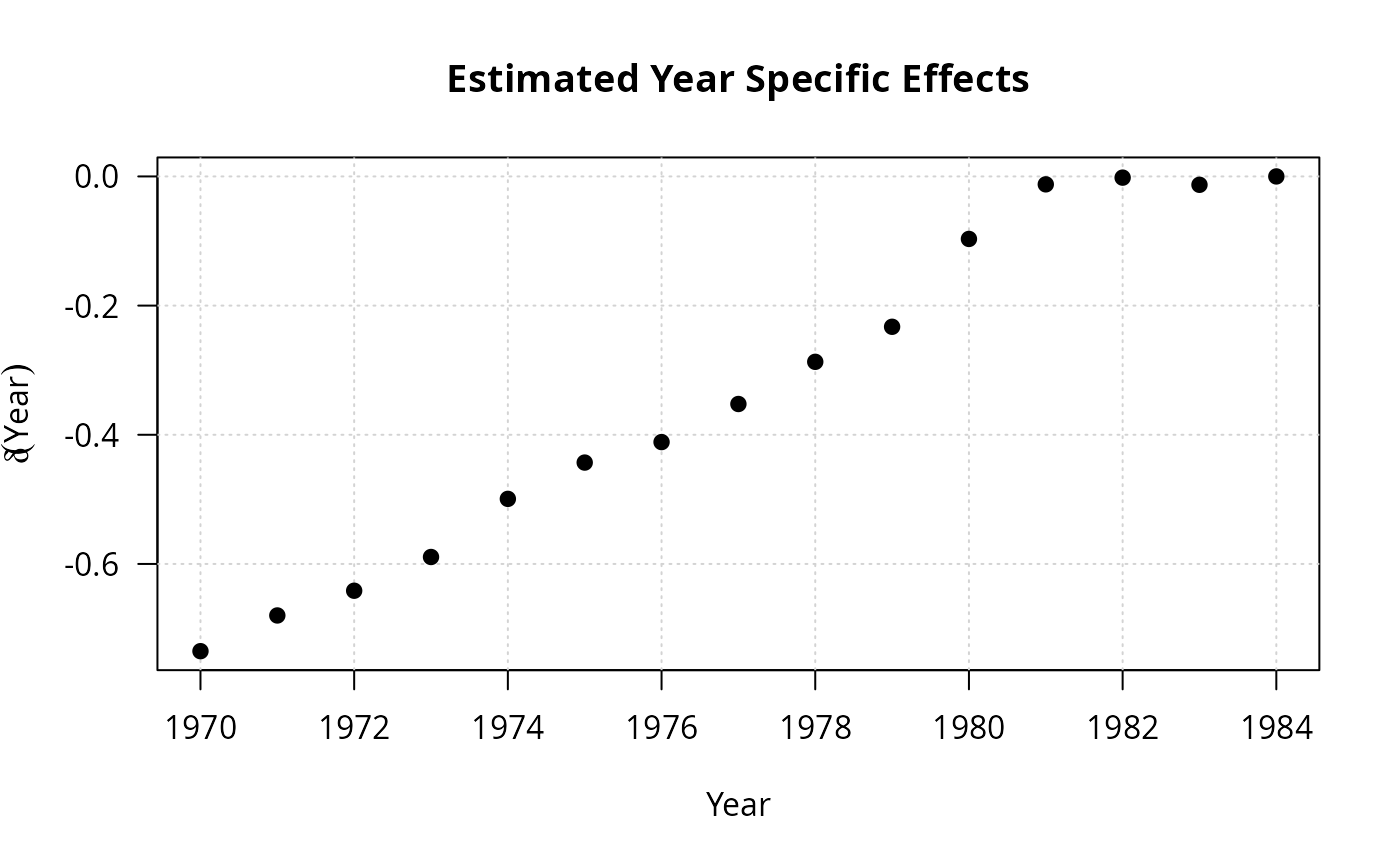 ## Table 7.2
anova(fm_full, fm_time)
#> Analysis of Variance Table
#>
#> Model 1: log(cost) ~ log(output) + I(log(output)^2) + log(price) + load +
#> year + firm
#> Model 2: log(cost) ~ log(output) + I(log(output)^2) + log(price) + load +
#> year
#> Res.Df RSS Df Sum of Sq F Pr(>F)
#> 1 66 0.17257
#> 2 71 1.03470 -5 -0.86213 65.945 < 2.2e-16 ***
#> ---
#> Signif. codes: 0 ‘***’ 0.001 ‘**’ 0.01 ‘*’ 0.05 ‘.’ 0.1 ‘ ’ 1
anova(fm_full, fm_firm)
#> Analysis of Variance Table
#>
#> Model 1: log(cost) ~ log(output) + I(log(output)^2) + log(price) + load +
#> year + firm
#> Model 2: log(cost) ~ log(output) + I(log(output)^2) + log(price) + load +
#> firm
#> Res.Df RSS Df Sum of Sq F Pr(>F)
#> 1 66 0.17257
#> 2 80 0.26815 -14 -0.095584 2.6112 0.004582 **
#> ---
#> Signif. codes: 0 ‘***’ 0.001 ‘**’ 0.01 ‘*’ 0.05 ‘.’ 0.1 ‘ ’ 1
anova(fm_full, fm_no)
#> Analysis of Variance Table
#>
#> Model 1: log(cost) ~ log(output) + I(log(output)^2) + log(price) + load +
#> year + firm
#> Model 2: log(cost) ~ log(output) + I(log(output)^2) + log(price) + load
#> Res.Df RSS Df Sum of Sq F Pr(>F)
#> 1 66 0.17257
#> 2 85 1.27492 -19 -1.1023 22.189 < 2.2e-16 ***
#> ---
#> Signif. codes: 0 ‘***’ 0.001 ‘**’ 0.01 ‘*’ 0.05 ‘.’ 0.1 ‘ ’ 1
## alternatively, use plm()
library("plm")
usair <- pdata.frame(USAirlines, c("firm", "year"))
fm_full2 <- plm(log(cost) ~ log(output) + I(log(output)^2) + log(price) + load,
data = usair, model = "within", effect = "twoways")
fm_time2 <- plm(log(cost) ~ log(output) + I(log(output)^2) + log(price) + load,
data = usair, model = "within", effect = "time")
fm_firm2 <- plm(log(cost) ~ log(output) + I(log(output)^2) + log(price) + load,
data = usair, model = "within", effect = "individual")
fm_no2 <- plm(log(cost) ~ log(output) + I(log(output)^2) + log(price) + load,
data = usair, model = "pooling")
pFtest(fm_full2, fm_time2)
#>
#> F test for twoways effects
#>
#> data: log(cost) ~ log(output) + I(log(output)^2) + log(price) + load
#> F = 65.945, df1 = 5, df2 = 66, p-value < 2.2e-16
#> alternative hypothesis: significant effects
#>
pFtest(fm_full2, fm_firm2)
#>
#> F test for twoways effects
#>
#> data: log(cost) ~ log(output) + I(log(output)^2) + log(price) + load
#> F = 2.6112, df1 = 14, df2 = 66, p-value = 0.004582
#> alternative hypothesis: significant effects
#>
pFtest(fm_full2, fm_no2)
#>
#> F test for twoways effects
#>
#> data: log(cost) ~ log(output) + I(log(output)^2) + log(price) + load
#> F = 22.189, df1 = 19, df2 = 66, p-value < 2.2e-16
#> alternative hypothesis: significant effects
#>
## Example 13.1, Table 13.1
fm_no <- plm(log(cost) ~ log(output) + log(price) + load, data = usair, model = "pooling")
fm_gm <- plm(log(cost) ~ log(output) + log(price) + load, data = usair, model = "between")
fm_firm <- plm(log(cost) ~ log(output) + log(price) + load, data = usair, model = "within")
fm_time <- plm(log(cost) ~ log(output) + log(price) + load, data = usair, model = "within",
effect = "time")
fm_ft <- plm(log(cost) ~ log(output) + log(price) + load, data = usair, model = "within",
effect = "twoways")
summary(fm_no)
#> Pooling Model
#>
#> Call:
#> plm(formula = log(cost) ~ log(output) + log(price) + load, data = usair,
#> model = "pooling")
#>
#> Balanced Panel: n = 6, T = 15, N = 90
#>
#> Residuals:
#> Min. 1st Qu. Median 3rd Qu. Max.
#> -0.2631215 -0.0575660 0.0044011 0.0850025 0.3001454
#>
#> Coefficients:
#> Estimate Std. Error t-value Pr(>|t|)
#> (Intercept) 9.516922 0.229245 41.5143 < 2.2e-16 ***
#> log(output) 0.882739 0.013255 66.5991 < 2.2e-16 ***
#> log(price) 0.453977 0.020304 22.3588 < 2.2e-16 ***
#> load -1.627510 0.345302 -4.7133 9.309e-06 ***
#> ---
#> Signif. codes: 0 ‘***’ 0.001 ‘**’ 0.01 ‘*’ 0.05 ‘.’ 0.1 ‘ ’ 1
#>
#> Total Sum of Squares: 114.04
#> Residual Sum of Squares: 1.3354
#> R-Squared: 0.98829
#> Adj. R-Squared: 0.98788
#> F-statistic: 2419.34 on 3 and 86 DF, p-value: < 2.22e-16
summary(fm_gm)
#> Oneway (individual) effect Between Model
#>
#> Call:
#> plm(formula = log(cost) ~ log(output) + log(price) + load, data = usair,
#> model = "between")
#>
#> Balanced Panel: n = 6, T = 15, N = 90
#> Observations used in estimation: 6
#>
#> Residuals:
#> 1 2 3 4 5 6
#> -0.0073057 -0.0125824 -0.0492504 0.1507977 -0.0023275 -0.0793316
#>
#> Coefficients:
#> Estimate Std. Error t-value Pr(>|t|)
#> (Intercept) 85.80867 56.48297 1.5192 0.26806
#> log(output) 0.78246 0.10877 7.1939 0.01878 *
#> log(price) -5.52395 4.47880 -1.2334 0.34273
#> load -1.75102 2.74319 -0.6383 0.58861
#> ---
#> Signif. codes: 0 ‘***’ 0.001 ‘**’ 0.01 ‘*’ 0.05 ‘.’ 0.1 ‘ ’ 1
#>
#> Total Sum of Squares: 4.9787
#> Residual Sum of Squares: 0.031676
#> R-Squared: 0.99364
#> Adj. R-Squared: 0.98409
#> F-statistic: 104.116 on 3 and 2 DF, p-value: 0.0095284
summary(fm_firm)
#> Oneway (individual) effect Within Model
#>
#> Call:
#> plm(formula = log(cost) ~ log(output) + log(price) + load, data = usair,
#> model = "within")
#>
#> Balanced Panel: n = 6, T = 15, N = 90
#>
#> Residuals:
#> Min. 1st Qu. Median 3rd Qu. Max.
#> -0.1560412 -0.0352173 -0.0093022 0.0349257 0.1658661
#>
#> Coefficients:
#> Estimate Std. Error t-value Pr(>|t|)
#> log(output) 0.919285 0.029890 30.7555 < 2e-16 ***
#> log(price) 0.417492 0.015199 27.4682 < 2e-16 ***
#> load -1.070396 0.201690 -5.3071 9.5e-07 ***
#> ---
#> Signif. codes: 0 ‘***’ 0.001 ‘**’ 0.01 ‘*’ 0.05 ‘.’ 0.1 ‘ ’ 1
#>
#> Total Sum of Squares: 39.361
#> Residual Sum of Squares: 0.29262
#> R-Squared: 0.99257
#> Adj. R-Squared: 0.99183
#> F-statistic: 3604.81 on 3 and 81 DF, p-value: < 2.22e-16
fixef(fm_firm)
#> 1 2 3 4 5 6
#> 9.7059 9.6647 9.4970 9.8905 9.7300 9.7930
summary(fm_time)
#> Oneway (time) effect Within Model
#>
#> Call:
#> plm(formula = log(cost) ~ log(output) + log(price) + load, data = usair,
#> effect = "time", model = "within")
#>
#> Balanced Panel: n = 6, T = 15, N = 90
#>
#> Residuals:
#> Min. 1st Qu. Median 3rd Qu. Max.
#> -0.2320007 -0.0587561 0.0046842 0.0487582 0.2871562
#>
#> Coefficients:
#> Estimate Std. Error t-value Pr(>|t|)
#> log(output) 0.867727 0.015408 56.3159 < 2.2e-16 ***
#> log(price) -0.484485 0.364109 -1.3306 0.1875
#> load -1.954403 0.442378 -4.4179 3.447e-05 ***
#> ---
#> Signif. codes: 0 ‘***’ 0.001 ‘**’ 0.01 ‘*’ 0.05 ‘.’ 0.1 ‘ ’ 1
#>
#> Total Sum of Squares: 76.734
#> Residual Sum of Squares: 1.0882
#> R-Squared: 0.98582
#> Adj. R-Squared: 0.98247
#> F-statistic: 1668.37 on 3 and 72 DF, p-value: < 2.22e-16
fixef(fm_time)
#> 1970 1971 1972 1973 1974 1975 1976 1977 1978 1979 1980
#> 20.496 20.578 20.656 20.741 21.200 21.412 21.503 21.654 21.830 22.114 22.465
#> 1981 1982 1983 1984
#> 22.651 22.617 22.552 22.537
summary(fm_ft)
#> Twoways effects Within Model
#>
#> Call:
#> plm(formula = log(cost) ~ log(output) + log(price) + load, data = usair,
#> effect = "twoways", model = "within")
#>
#> Balanced Panel: n = 6, T = 15, N = 90
#>
#> Residuals:
#> Min. 1st Qu. Median 3rd Qu. Max.
#> -0.123460 -0.024922 0.001185 0.024570 0.132182
#>
#> Coefficients:
#> Estimate Std. Error t-value Pr(>|t|)
#> log(output) 0.817249 0.031851 25.6586 < 2.2e-16 ***
#> log(price) 0.168611 0.163478 1.0314 0.306064
#> load -0.882812 0.261737 -3.3729 0.001239 **
#> ---
#> Signif. codes: 0 ‘***’ 0.001 ‘**’ 0.01 ‘*’ 0.05 ‘.’ 0.1 ‘ ’ 1
#>
#> Total Sum of Squares: 2.0542
#> Residual Sum of Squares: 0.17685
#> R-Squared: 0.91391
#> Adj. R-Squared: 0.88564
#> F-statistic: 237.088 on 3 and 67 DF, p-value: < 2.22e-16
fixef(fm_ft, effect = "individual")
#> 1 2 3 4 5 6
#> 12.421 12.358 12.103 12.427 12.200 12.247
fixef(fm_ft, effect = "time")
#> 1970 1971 1972 1973 1974 1975 1976 1977 1978 1979 1980
#> 12.421 12.476 12.519 12.572 12.641 12.687 12.718 12.774 12.842 12.887 13.003
#> 1981 1982 1983 1984
#> 13.081 13.097 13.096 13.114
## Table 13.2
fm_rfirm <- plm(log(cost) ~ log(output) + log(price) + load, data = usair, model = "random")
fm_rft <- plm(log(cost) ~ log(output) + log(price) + load, data = usair, model = "random",
effect = "twoways")
summary(fm_rfirm)
#> Oneway (individual) effect Random Effect Model
#> (Swamy-Arora's transformation)
#>
#> Call:
#> plm(formula = log(cost) ~ log(output) + log(price) + load, data = usair,
#> model = "random")
#>
#> Balanced Panel: n = 6, T = 15, N = 90
#>
#> Effects:
#> var std.dev share
#> idiosyncratic 0.003613 0.060105 0.188
#> individual 0.015597 0.124889 0.812
#> theta: 0.8767
#>
#> Residuals:
#> Min. 1st Qu. Median 3rd Qu. Max.
#> -0.1385541 -0.0390391 -0.0045664 0.0365641 0.1774947
#>
#> Coefficients:
#> Estimate Std. Error z-value Pr(>|z|)
#> (Intercept) 9.627909 0.210164 45.8114 < 2.2e-16 ***
#> log(output) 0.906681 0.025625 35.3827 < 2.2e-16 ***
#> log(price) 0.422778 0.014025 30.1451 < 2.2e-16 ***
#> load -1.064498 0.200070 -5.3206 1.034e-07 ***
#> ---
#> Signif. codes: 0 ‘***’ 0.001 ‘**’ 0.01 ‘*’ 0.05 ‘.’ 0.1 ‘ ’ 1
#>
#> Total Sum of Squares: 40.497
#> Residual Sum of Squares: 0.31159
#> R-Squared: 0.99231
#> Adj. R-Squared: 0.99204
#> Chisq: 11091.4 on 3 DF, p-value: < 2.22e-16
summary(fm_rft)
#> Twoways effects Random Effect Model
#> (Swamy-Arora's transformation)
#>
#> Call:
#> plm(formula = log(cost) ~ log(output) + log(price) + load, data = usair,
#> effect = "twoways", model = "random")
#>
#> Balanced Panel: n = 6, T = 15, N = 90
#>
#> Effects:
#> var std.dev share
#> idiosyncratic 2.640e-03 5.138e-02 0.144
#> individual 1.566e-02 1.251e-01 0.853
#> time 6.831e-05 8.265e-03 0.004
#> theta: 0.8946 (id) 0.06963 (time) 0.06954 (total)
#>
#> Residuals:
#> Min. 1st Qu. Median 3rd Qu. Max.
#> -0.1392549 -0.0379739 -0.0040778 0.0361744 0.1726892
#>
#> Coefficients:
#> Estimate Std. Error z-value Pr(>|z|)
#> (Intercept) 9.598602 0.217634 44.1043 < 2.2e-16 ***
#> log(output) 0.902373 0.026252 34.3738 < 2.2e-16 ***
#> log(price) 0.424178 0.014392 29.4723 < 2.2e-16 ***
#> load -1.053130 0.202555 -5.1992 2.001e-07 ***
#> ---
#> Signif. codes: 0 ‘***’ 0.001 ‘**’ 0.01 ‘*’ 0.05 ‘.’ 0.1 ‘ ’ 1
#>
#> Total Sum of Squares: 35.176
#> Residual Sum of Squares: 0.29403
#> R-Squared: 0.99164
#> Adj. R-Squared: 0.99135
#> Chisq: 10202.5 on 3 DF, p-value: < 2.22e-16
#################################################
## Cost function of electricity producers 1955 ##
#################################################
## Nerlove data
data("Electricity1955", package = "AER")
Electricity <- Electricity1955[1:145,]
## Example 7.3
## Cobb-Douglas cost function
fm_all <- lm(log(cost/fuel) ~ log(output) + log(labor/fuel) + log(capital/fuel),
data = Electricity)
summary(fm_all)
#>
#> Call:
#> lm(formula = log(cost/fuel) ~ log(output) + log(labor/fuel) +
#> log(capital/fuel), data = Electricity)
#>
#> Residuals:
#> Min 1Q Median 3Q Max
#> -1.01212 -0.21789 -0.00753 0.16046 1.81898
#>
#> Coefficients:
#> Estimate Std. Error t value Pr(>|t|)
#> (Intercept) -4.685776 0.885294 -5.293 4.51e-07 ***
#> log(output) 0.720667 0.017435 41.335 < 2e-16 ***
#> log(labor/fuel) 0.593972 0.204632 2.903 0.0043 **
#> log(capital/fuel) -0.008471 0.190842 -0.044 0.9647
#> ---
#> Signif. codes: 0 ‘***’ 0.001 ‘**’ 0.01 ‘*’ 0.05 ‘.’ 0.1 ‘ ’ 1
#>
#> Residual standard error: 0.3917 on 141 degrees of freedom
#> Multiple R-squared: 0.9316, Adjusted R-squared: 0.9301
#> F-statistic: 640.1 on 3 and 141 DF, p-value: < 2.2e-16
#>
## hypothesis of constant returns to scale
linearHypothesis(fm_all, "log(output) = 1")
#>
#> Linear hypothesis test:
#> log(output) = 1
#>
#> Model 1: restricted model
#> Model 2: log(cost/fuel) ~ log(output) + log(labor/fuel) + log(capital/fuel)
#>
#> Res.Df RSS Df Sum of Sq F Pr(>F)
#> 1 142 61.027
#> 2 141 21.637 1 39.39 256.69 < 2.2e-16 ***
#> ---
#> Signif. codes: 0 ‘***’ 0.001 ‘**’ 0.01 ‘*’ 0.05 ‘.’ 0.1 ‘ ’ 1
## Figure 7.4
plot(residuals(fm_all) ~ log(output), data = Electricity)
## Table 7.2
anova(fm_full, fm_time)
#> Analysis of Variance Table
#>
#> Model 1: log(cost) ~ log(output) + I(log(output)^2) + log(price) + load +
#> year + firm
#> Model 2: log(cost) ~ log(output) + I(log(output)^2) + log(price) + load +
#> year
#> Res.Df RSS Df Sum of Sq F Pr(>F)
#> 1 66 0.17257
#> 2 71 1.03470 -5 -0.86213 65.945 < 2.2e-16 ***
#> ---
#> Signif. codes: 0 ‘***’ 0.001 ‘**’ 0.01 ‘*’ 0.05 ‘.’ 0.1 ‘ ’ 1
anova(fm_full, fm_firm)
#> Analysis of Variance Table
#>
#> Model 1: log(cost) ~ log(output) + I(log(output)^2) + log(price) + load +
#> year + firm
#> Model 2: log(cost) ~ log(output) + I(log(output)^2) + log(price) + load +
#> firm
#> Res.Df RSS Df Sum of Sq F Pr(>F)
#> 1 66 0.17257
#> 2 80 0.26815 -14 -0.095584 2.6112 0.004582 **
#> ---
#> Signif. codes: 0 ‘***’ 0.001 ‘**’ 0.01 ‘*’ 0.05 ‘.’ 0.1 ‘ ’ 1
anova(fm_full, fm_no)
#> Analysis of Variance Table
#>
#> Model 1: log(cost) ~ log(output) + I(log(output)^2) + log(price) + load +
#> year + firm
#> Model 2: log(cost) ~ log(output) + I(log(output)^2) + log(price) + load
#> Res.Df RSS Df Sum of Sq F Pr(>F)
#> 1 66 0.17257
#> 2 85 1.27492 -19 -1.1023 22.189 < 2.2e-16 ***
#> ---
#> Signif. codes: 0 ‘***’ 0.001 ‘**’ 0.01 ‘*’ 0.05 ‘.’ 0.1 ‘ ’ 1
## alternatively, use plm()
library("plm")
usair <- pdata.frame(USAirlines, c("firm", "year"))
fm_full2 <- plm(log(cost) ~ log(output) + I(log(output)^2) + log(price) + load,
data = usair, model = "within", effect = "twoways")
fm_time2 <- plm(log(cost) ~ log(output) + I(log(output)^2) + log(price) + load,
data = usair, model = "within", effect = "time")
fm_firm2 <- plm(log(cost) ~ log(output) + I(log(output)^2) + log(price) + load,
data = usair, model = "within", effect = "individual")
fm_no2 <- plm(log(cost) ~ log(output) + I(log(output)^2) + log(price) + load,
data = usair, model = "pooling")
pFtest(fm_full2, fm_time2)
#>
#> F test for twoways effects
#>
#> data: log(cost) ~ log(output) + I(log(output)^2) + log(price) + load
#> F = 65.945, df1 = 5, df2 = 66, p-value < 2.2e-16
#> alternative hypothesis: significant effects
#>
pFtest(fm_full2, fm_firm2)
#>
#> F test for twoways effects
#>
#> data: log(cost) ~ log(output) + I(log(output)^2) + log(price) + load
#> F = 2.6112, df1 = 14, df2 = 66, p-value = 0.004582
#> alternative hypothesis: significant effects
#>
pFtest(fm_full2, fm_no2)
#>
#> F test for twoways effects
#>
#> data: log(cost) ~ log(output) + I(log(output)^2) + log(price) + load
#> F = 22.189, df1 = 19, df2 = 66, p-value < 2.2e-16
#> alternative hypothesis: significant effects
#>
## Example 13.1, Table 13.1
fm_no <- plm(log(cost) ~ log(output) + log(price) + load, data = usair, model = "pooling")
fm_gm <- plm(log(cost) ~ log(output) + log(price) + load, data = usair, model = "between")
fm_firm <- plm(log(cost) ~ log(output) + log(price) + load, data = usair, model = "within")
fm_time <- plm(log(cost) ~ log(output) + log(price) + load, data = usair, model = "within",
effect = "time")
fm_ft <- plm(log(cost) ~ log(output) + log(price) + load, data = usair, model = "within",
effect = "twoways")
summary(fm_no)
#> Pooling Model
#>
#> Call:
#> plm(formula = log(cost) ~ log(output) + log(price) + load, data = usair,
#> model = "pooling")
#>
#> Balanced Panel: n = 6, T = 15, N = 90
#>
#> Residuals:
#> Min. 1st Qu. Median 3rd Qu. Max.
#> -0.2631215 -0.0575660 0.0044011 0.0850025 0.3001454
#>
#> Coefficients:
#> Estimate Std. Error t-value Pr(>|t|)
#> (Intercept) 9.516922 0.229245 41.5143 < 2.2e-16 ***
#> log(output) 0.882739 0.013255 66.5991 < 2.2e-16 ***
#> log(price) 0.453977 0.020304 22.3588 < 2.2e-16 ***
#> load -1.627510 0.345302 -4.7133 9.309e-06 ***
#> ---
#> Signif. codes: 0 ‘***’ 0.001 ‘**’ 0.01 ‘*’ 0.05 ‘.’ 0.1 ‘ ’ 1
#>
#> Total Sum of Squares: 114.04
#> Residual Sum of Squares: 1.3354
#> R-Squared: 0.98829
#> Adj. R-Squared: 0.98788
#> F-statistic: 2419.34 on 3 and 86 DF, p-value: < 2.22e-16
summary(fm_gm)
#> Oneway (individual) effect Between Model
#>
#> Call:
#> plm(formula = log(cost) ~ log(output) + log(price) + load, data = usair,
#> model = "between")
#>
#> Balanced Panel: n = 6, T = 15, N = 90
#> Observations used in estimation: 6
#>
#> Residuals:
#> 1 2 3 4 5 6
#> -0.0073057 -0.0125824 -0.0492504 0.1507977 -0.0023275 -0.0793316
#>
#> Coefficients:
#> Estimate Std. Error t-value Pr(>|t|)
#> (Intercept) 85.80867 56.48297 1.5192 0.26806
#> log(output) 0.78246 0.10877 7.1939 0.01878 *
#> log(price) -5.52395 4.47880 -1.2334 0.34273
#> load -1.75102 2.74319 -0.6383 0.58861
#> ---
#> Signif. codes: 0 ‘***’ 0.001 ‘**’ 0.01 ‘*’ 0.05 ‘.’ 0.1 ‘ ’ 1
#>
#> Total Sum of Squares: 4.9787
#> Residual Sum of Squares: 0.031676
#> R-Squared: 0.99364
#> Adj. R-Squared: 0.98409
#> F-statistic: 104.116 on 3 and 2 DF, p-value: 0.0095284
summary(fm_firm)
#> Oneway (individual) effect Within Model
#>
#> Call:
#> plm(formula = log(cost) ~ log(output) + log(price) + load, data = usair,
#> model = "within")
#>
#> Balanced Panel: n = 6, T = 15, N = 90
#>
#> Residuals:
#> Min. 1st Qu. Median 3rd Qu. Max.
#> -0.1560412 -0.0352173 -0.0093022 0.0349257 0.1658661
#>
#> Coefficients:
#> Estimate Std. Error t-value Pr(>|t|)
#> log(output) 0.919285 0.029890 30.7555 < 2e-16 ***
#> log(price) 0.417492 0.015199 27.4682 < 2e-16 ***
#> load -1.070396 0.201690 -5.3071 9.5e-07 ***
#> ---
#> Signif. codes: 0 ‘***’ 0.001 ‘**’ 0.01 ‘*’ 0.05 ‘.’ 0.1 ‘ ’ 1
#>
#> Total Sum of Squares: 39.361
#> Residual Sum of Squares: 0.29262
#> R-Squared: 0.99257
#> Adj. R-Squared: 0.99183
#> F-statistic: 3604.81 on 3 and 81 DF, p-value: < 2.22e-16
fixef(fm_firm)
#> 1 2 3 4 5 6
#> 9.7059 9.6647 9.4970 9.8905 9.7300 9.7930
summary(fm_time)
#> Oneway (time) effect Within Model
#>
#> Call:
#> plm(formula = log(cost) ~ log(output) + log(price) + load, data = usair,
#> effect = "time", model = "within")
#>
#> Balanced Panel: n = 6, T = 15, N = 90
#>
#> Residuals:
#> Min. 1st Qu. Median 3rd Qu. Max.
#> -0.2320007 -0.0587561 0.0046842 0.0487582 0.2871562
#>
#> Coefficients:
#> Estimate Std. Error t-value Pr(>|t|)
#> log(output) 0.867727 0.015408 56.3159 < 2.2e-16 ***
#> log(price) -0.484485 0.364109 -1.3306 0.1875
#> load -1.954403 0.442378 -4.4179 3.447e-05 ***
#> ---
#> Signif. codes: 0 ‘***’ 0.001 ‘**’ 0.01 ‘*’ 0.05 ‘.’ 0.1 ‘ ’ 1
#>
#> Total Sum of Squares: 76.734
#> Residual Sum of Squares: 1.0882
#> R-Squared: 0.98582
#> Adj. R-Squared: 0.98247
#> F-statistic: 1668.37 on 3 and 72 DF, p-value: < 2.22e-16
fixef(fm_time)
#> 1970 1971 1972 1973 1974 1975 1976 1977 1978 1979 1980
#> 20.496 20.578 20.656 20.741 21.200 21.412 21.503 21.654 21.830 22.114 22.465
#> 1981 1982 1983 1984
#> 22.651 22.617 22.552 22.537
summary(fm_ft)
#> Twoways effects Within Model
#>
#> Call:
#> plm(formula = log(cost) ~ log(output) + log(price) + load, data = usair,
#> effect = "twoways", model = "within")
#>
#> Balanced Panel: n = 6, T = 15, N = 90
#>
#> Residuals:
#> Min. 1st Qu. Median 3rd Qu. Max.
#> -0.123460 -0.024922 0.001185 0.024570 0.132182
#>
#> Coefficients:
#> Estimate Std. Error t-value Pr(>|t|)
#> log(output) 0.817249 0.031851 25.6586 < 2.2e-16 ***
#> log(price) 0.168611 0.163478 1.0314 0.306064
#> load -0.882812 0.261737 -3.3729 0.001239 **
#> ---
#> Signif. codes: 0 ‘***’ 0.001 ‘**’ 0.01 ‘*’ 0.05 ‘.’ 0.1 ‘ ’ 1
#>
#> Total Sum of Squares: 2.0542
#> Residual Sum of Squares: 0.17685
#> R-Squared: 0.91391
#> Adj. R-Squared: 0.88564
#> F-statistic: 237.088 on 3 and 67 DF, p-value: < 2.22e-16
fixef(fm_ft, effect = "individual")
#> 1 2 3 4 5 6
#> 12.421 12.358 12.103 12.427 12.200 12.247
fixef(fm_ft, effect = "time")
#> 1970 1971 1972 1973 1974 1975 1976 1977 1978 1979 1980
#> 12.421 12.476 12.519 12.572 12.641 12.687 12.718 12.774 12.842 12.887 13.003
#> 1981 1982 1983 1984
#> 13.081 13.097 13.096 13.114
## Table 13.2
fm_rfirm <- plm(log(cost) ~ log(output) + log(price) + load, data = usair, model = "random")
fm_rft <- plm(log(cost) ~ log(output) + log(price) + load, data = usair, model = "random",
effect = "twoways")
summary(fm_rfirm)
#> Oneway (individual) effect Random Effect Model
#> (Swamy-Arora's transformation)
#>
#> Call:
#> plm(formula = log(cost) ~ log(output) + log(price) + load, data = usair,
#> model = "random")
#>
#> Balanced Panel: n = 6, T = 15, N = 90
#>
#> Effects:
#> var std.dev share
#> idiosyncratic 0.003613 0.060105 0.188
#> individual 0.015597 0.124889 0.812
#> theta: 0.8767
#>
#> Residuals:
#> Min. 1st Qu. Median 3rd Qu. Max.
#> -0.1385541 -0.0390391 -0.0045664 0.0365641 0.1774947
#>
#> Coefficients:
#> Estimate Std. Error z-value Pr(>|z|)
#> (Intercept) 9.627909 0.210164 45.8114 < 2.2e-16 ***
#> log(output) 0.906681 0.025625 35.3827 < 2.2e-16 ***
#> log(price) 0.422778 0.014025 30.1451 < 2.2e-16 ***
#> load -1.064498 0.200070 -5.3206 1.034e-07 ***
#> ---
#> Signif. codes: 0 ‘***’ 0.001 ‘**’ 0.01 ‘*’ 0.05 ‘.’ 0.1 ‘ ’ 1
#>
#> Total Sum of Squares: 40.497
#> Residual Sum of Squares: 0.31159
#> R-Squared: 0.99231
#> Adj. R-Squared: 0.99204
#> Chisq: 11091.4 on 3 DF, p-value: < 2.22e-16
summary(fm_rft)
#> Twoways effects Random Effect Model
#> (Swamy-Arora's transformation)
#>
#> Call:
#> plm(formula = log(cost) ~ log(output) + log(price) + load, data = usair,
#> effect = "twoways", model = "random")
#>
#> Balanced Panel: n = 6, T = 15, N = 90
#>
#> Effects:
#> var std.dev share
#> idiosyncratic 2.640e-03 5.138e-02 0.144
#> individual 1.566e-02 1.251e-01 0.853
#> time 6.831e-05 8.265e-03 0.004
#> theta: 0.8946 (id) 0.06963 (time) 0.06954 (total)
#>
#> Residuals:
#> Min. 1st Qu. Median 3rd Qu. Max.
#> -0.1392549 -0.0379739 -0.0040778 0.0361744 0.1726892
#>
#> Coefficients:
#> Estimate Std. Error z-value Pr(>|z|)
#> (Intercept) 9.598602 0.217634 44.1043 < 2.2e-16 ***
#> log(output) 0.902373 0.026252 34.3738 < 2.2e-16 ***
#> log(price) 0.424178 0.014392 29.4723 < 2.2e-16 ***
#> load -1.053130 0.202555 -5.1992 2.001e-07 ***
#> ---
#> Signif. codes: 0 ‘***’ 0.001 ‘**’ 0.01 ‘*’ 0.05 ‘.’ 0.1 ‘ ’ 1
#>
#> Total Sum of Squares: 35.176
#> Residual Sum of Squares: 0.29403
#> R-Squared: 0.99164
#> Adj. R-Squared: 0.99135
#> Chisq: 10202.5 on 3 DF, p-value: < 2.22e-16
#################################################
## Cost function of electricity producers 1955 ##
#################################################
## Nerlove data
data("Electricity1955", package = "AER")
Electricity <- Electricity1955[1:145,]
## Example 7.3
## Cobb-Douglas cost function
fm_all <- lm(log(cost/fuel) ~ log(output) + log(labor/fuel) + log(capital/fuel),
data = Electricity)
summary(fm_all)
#>
#> Call:
#> lm(formula = log(cost/fuel) ~ log(output) + log(labor/fuel) +
#> log(capital/fuel), data = Electricity)
#>
#> Residuals:
#> Min 1Q Median 3Q Max
#> -1.01212 -0.21789 -0.00753 0.16046 1.81898
#>
#> Coefficients:
#> Estimate Std. Error t value Pr(>|t|)
#> (Intercept) -4.685776 0.885294 -5.293 4.51e-07 ***
#> log(output) 0.720667 0.017435 41.335 < 2e-16 ***
#> log(labor/fuel) 0.593972 0.204632 2.903 0.0043 **
#> log(capital/fuel) -0.008471 0.190842 -0.044 0.9647
#> ---
#> Signif. codes: 0 ‘***’ 0.001 ‘**’ 0.01 ‘*’ 0.05 ‘.’ 0.1 ‘ ’ 1
#>
#> Residual standard error: 0.3917 on 141 degrees of freedom
#> Multiple R-squared: 0.9316, Adjusted R-squared: 0.9301
#> F-statistic: 640.1 on 3 and 141 DF, p-value: < 2.2e-16
#>
## hypothesis of constant returns to scale
linearHypothesis(fm_all, "log(output) = 1")
#>
#> Linear hypothesis test:
#> log(output) = 1
#>
#> Model 1: restricted model
#> Model 2: log(cost/fuel) ~ log(output) + log(labor/fuel) + log(capital/fuel)
#>
#> Res.Df RSS Df Sum of Sq F Pr(>F)
#> 1 142 61.027
#> 2 141 21.637 1 39.39 256.69 < 2.2e-16 ***
#> ---
#> Signif. codes: 0 ‘***’ 0.001 ‘**’ 0.01 ‘*’ 0.05 ‘.’ 0.1 ‘ ’ 1
## Figure 7.4
plot(residuals(fm_all) ~ log(output), data = Electricity)
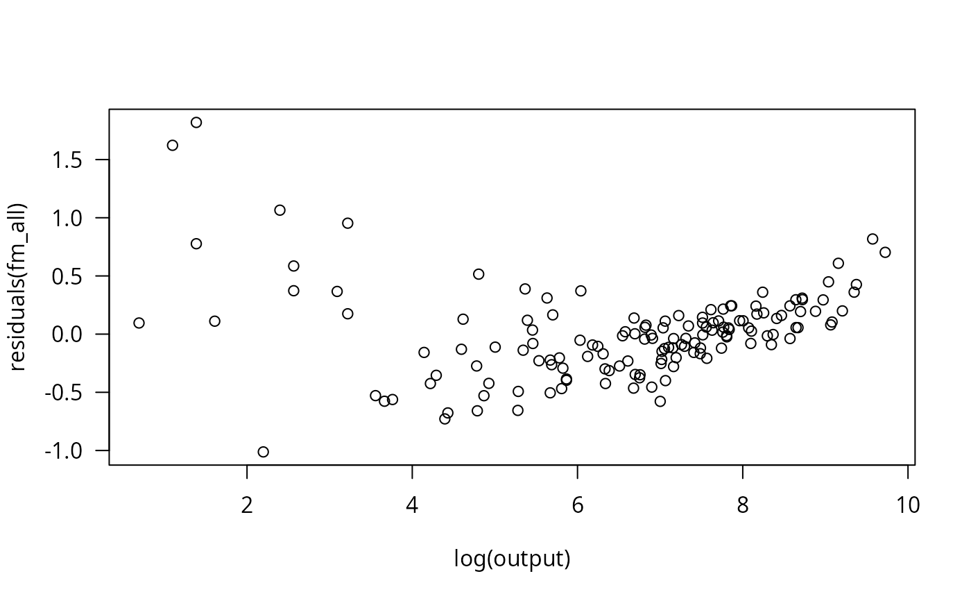 ## scaling seems to be different in Greene (2003) with logQ > 10?
## grouped functions
Electricity$group <- with(Electricity, cut(log(output), quantile(log(output), 0:5/5),
include.lowest = TRUE, labels = 1:5))
fm_group <- lm(
log(cost/fuel) ~ group/(log(output) + log(labor/fuel) + log(capital/fuel)) - 1,
data = Electricity)
## Table 7.3 (close, but not quite)
round(rbind(coef(fm_all)[-1], matrix(coef(fm_group), nrow = 5)[,-1]), digits = 3)
#> log(output) log(labor/fuel) log(capital/fuel)
#> [1,] 0.721 0.594 -0.008
#> [2,] 0.400 0.615 -0.081
#> [3,] 0.658 0.095 0.377
#> [4,] 0.938 0.402 0.250
#> [5,] 0.912 0.507 0.093
#> [6,] 1.044 0.603 -0.289
## Table 7.4
## log quadratic cost function
fm_all2 <- lm(
log(cost/fuel) ~ log(output) + I(log(output)^2) + log(labor/fuel) + log(capital/fuel),
data = Electricity)
summary(fm_all2)
#>
#> Call:
#> lm(formula = log(cost/fuel) ~ log(output) + I(log(output)^2) +
#> log(labor/fuel) + log(capital/fuel), data = Electricity)
#>
#> Residuals:
#> Min 1Q Median 3Q Max
#> -1.3825 -0.1373 0.0080 0.1277 1.1354
#>
#> Coefficients:
#> Estimate Std. Error t value Pr(>|t|)
#> (Intercept) -3.764003 0.702060 -5.361 3.32e-07 ***
#> log(output) 0.152648 0.061862 2.468 0.01481 *
#> I(log(output)^2) 0.050504 0.005364 9.415 < 2e-16 ***
#> log(labor/fuel) 0.480699 0.161142 2.983 0.00337 **
#> log(capital/fuel) 0.073897 0.150119 0.492 0.62331
#> ---
#> Signif. codes: 0 ‘***’ 0.001 ‘**’ 0.01 ‘*’ 0.05 ‘.’ 0.1 ‘ ’ 1
#>
#> Residual standard error: 0.3076 on 140 degrees of freedom
#> Multiple R-squared: 0.9581, Adjusted R-squared: 0.9569
#> F-statistic: 800.7 on 4 and 140 DF, p-value: < 2.2e-16
#>
##########################
## Technological change ##
##########################
## Exercise 7.1
data("TechChange", package = "AER")
fm1 <- lm(I(output/technology) ~ log(clr), data = TechChange)
fm2 <- lm(I(output/technology) ~ I(1/clr), data = TechChange)
fm3 <- lm(log(output/technology) ~ log(clr), data = TechChange)
fm4 <- lm(log(output/technology) ~ I(1/clr), data = TechChange)
## Exercise 7.2 (a) and (c)
plot(I(output/technology) ~ clr, data = TechChange)
## scaling seems to be different in Greene (2003) with logQ > 10?
## grouped functions
Electricity$group <- with(Electricity, cut(log(output), quantile(log(output), 0:5/5),
include.lowest = TRUE, labels = 1:5))
fm_group <- lm(
log(cost/fuel) ~ group/(log(output) + log(labor/fuel) + log(capital/fuel)) - 1,
data = Electricity)
## Table 7.3 (close, but not quite)
round(rbind(coef(fm_all)[-1], matrix(coef(fm_group), nrow = 5)[,-1]), digits = 3)
#> log(output) log(labor/fuel) log(capital/fuel)
#> [1,] 0.721 0.594 -0.008
#> [2,] 0.400 0.615 -0.081
#> [3,] 0.658 0.095 0.377
#> [4,] 0.938 0.402 0.250
#> [5,] 0.912 0.507 0.093
#> [6,] 1.044 0.603 -0.289
## Table 7.4
## log quadratic cost function
fm_all2 <- lm(
log(cost/fuel) ~ log(output) + I(log(output)^2) + log(labor/fuel) + log(capital/fuel),
data = Electricity)
summary(fm_all2)
#>
#> Call:
#> lm(formula = log(cost/fuel) ~ log(output) + I(log(output)^2) +
#> log(labor/fuel) + log(capital/fuel), data = Electricity)
#>
#> Residuals:
#> Min 1Q Median 3Q Max
#> -1.3825 -0.1373 0.0080 0.1277 1.1354
#>
#> Coefficients:
#> Estimate Std. Error t value Pr(>|t|)
#> (Intercept) -3.764003 0.702060 -5.361 3.32e-07 ***
#> log(output) 0.152648 0.061862 2.468 0.01481 *
#> I(log(output)^2) 0.050504 0.005364 9.415 < 2e-16 ***
#> log(labor/fuel) 0.480699 0.161142 2.983 0.00337 **
#> log(capital/fuel) 0.073897 0.150119 0.492 0.62331
#> ---
#> Signif. codes: 0 ‘***’ 0.001 ‘**’ 0.01 ‘*’ 0.05 ‘.’ 0.1 ‘ ’ 1
#>
#> Residual standard error: 0.3076 on 140 degrees of freedom
#> Multiple R-squared: 0.9581, Adjusted R-squared: 0.9569
#> F-statistic: 800.7 on 4 and 140 DF, p-value: < 2.2e-16
#>
##########################
## Technological change ##
##########################
## Exercise 7.1
data("TechChange", package = "AER")
fm1 <- lm(I(output/technology) ~ log(clr), data = TechChange)
fm2 <- lm(I(output/technology) ~ I(1/clr), data = TechChange)
fm3 <- lm(log(output/technology) ~ log(clr), data = TechChange)
fm4 <- lm(log(output/technology) ~ I(1/clr), data = TechChange)
## Exercise 7.2 (a) and (c)
plot(I(output/technology) ~ clr, data = TechChange)
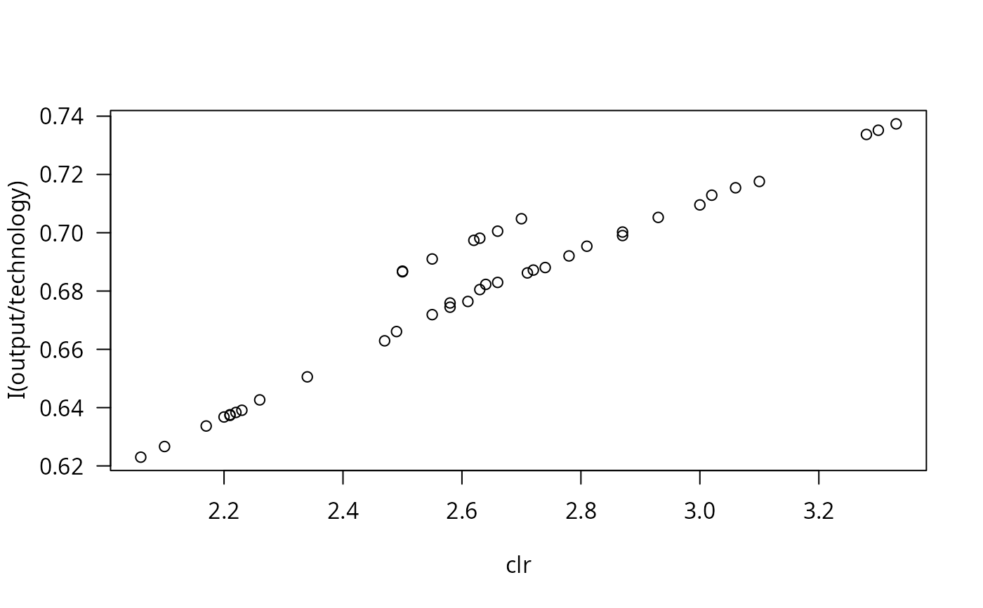 sctest(I(output/technology) ~ log(clr), data = TechChange,
type = "Chow", point = c(1942, 1))
#>
#> Chow test
#>
#> data: I(output/technology) ~ log(clr)
#> F = 1208.3, p-value < 2.2e-16
#>
##################################
## Expenditure and default data ##
##################################
## full data set (F21.4)
data("CreditCard", package = "AER")
## extract data set F9.1
ccard <- CreditCard[1:100,]
ccard$income <- round(ccard$income, digits = 2)
ccard$expenditure <- round(ccard$expenditure, digits = 2)
ccard$age <- round(ccard$age + .01)
## suspicious:
CreditCard$age[CreditCard$age < 1]
#> [1] 0.5000000 0.1666667 0.5833333 0.7500000 0.5833333 0.5000000 0.7500000
## the first of these is also in TableF9.1 with 36 instead of 0.5:
ccard$age[79] <- 36
## Example 11.1
ccard <- ccard[order(ccard$income),]
ccard0 <- subset(ccard, expenditure > 0)
cc_ols <- lm(expenditure ~ age + owner + income + I(income^2), data = ccard0)
## Figure 11.1
plot(residuals(cc_ols) ~ income, data = ccard0, pch = 19)
sctest(I(output/technology) ~ log(clr), data = TechChange,
type = "Chow", point = c(1942, 1))
#>
#> Chow test
#>
#> data: I(output/technology) ~ log(clr)
#> F = 1208.3, p-value < 2.2e-16
#>
##################################
## Expenditure and default data ##
##################################
## full data set (F21.4)
data("CreditCard", package = "AER")
## extract data set F9.1
ccard <- CreditCard[1:100,]
ccard$income <- round(ccard$income, digits = 2)
ccard$expenditure <- round(ccard$expenditure, digits = 2)
ccard$age <- round(ccard$age + .01)
## suspicious:
CreditCard$age[CreditCard$age < 1]
#> [1] 0.5000000 0.1666667 0.5833333 0.7500000 0.5833333 0.5000000 0.7500000
## the first of these is also in TableF9.1 with 36 instead of 0.5:
ccard$age[79] <- 36
## Example 11.1
ccard <- ccard[order(ccard$income),]
ccard0 <- subset(ccard, expenditure > 0)
cc_ols <- lm(expenditure ~ age + owner + income + I(income^2), data = ccard0)
## Figure 11.1
plot(residuals(cc_ols) ~ income, data = ccard0, pch = 19)
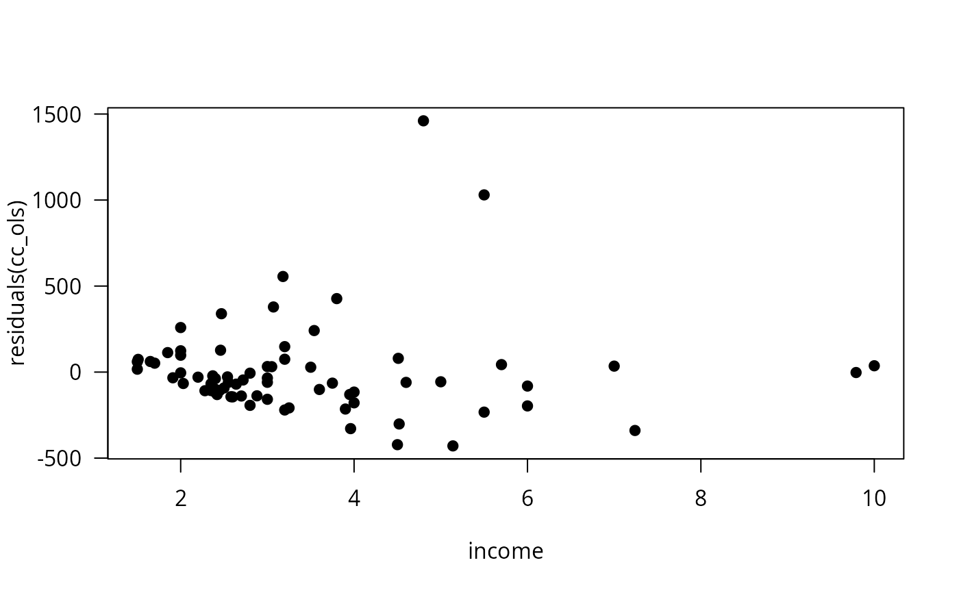 ## Table 11.1
mean(ccard$age)
#> [1] 32.08
prop.table(table(ccard$owner))
#>
#> no yes
#> 0.64 0.36
mean(ccard$income)
#> [1] 3.3692
summary(cc_ols)
#>
#> Call:
#> lm(formula = expenditure ~ age + owner + income + I(income^2),
#> data = ccard0)
#>
#> Residuals:
#> Min 1Q Median 3Q Max
#> -429.03 -130.39 -51.14 53.96 1460.55
#>
#> Coefficients:
#> Estimate Std. Error t value Pr(>|t|)
#> (Intercept) -237.127 199.324 -1.190 0.23838
#> age -3.086 5.515 -0.560 0.57759
#> owneryes 27.911 82.920 0.337 0.73747
#> income 234.416 80.365 2.917 0.00481 **
#> I(income^2) -15.002 7.469 -2.009 0.04861 *
#> ---
#> Signif. codes: 0 ‘***’ 0.001 ‘**’ 0.01 ‘*’ 0.05 ‘.’ 0.1 ‘ ’ 1
#>
#> Residual standard error: 284.7 on 67 degrees of freedom
#> Multiple R-squared: 0.2436, Adjusted R-squared: 0.1985
#> F-statistic: 5.396 on 4 and 67 DF, p-value: 0.0007932
#>
sqrt(diag(vcovHC(cc_ols, type = "HC0")))
#> (Intercept) age owneryes income I(income^2)
#> 212.953161 3.300911 92.190987 88.874353 6.945292
sqrt(diag(vcovHC(cc_ols, type = "HC2")))
#> (Intercept) age owneryes income I(income^2)
#> 221.050557 3.446920 95.675689 92.092471 7.200369
sqrt(diag(vcovHC(cc_ols, type = "HC1")))
#> (Intercept) age owneryes income I(income^2)
#> 220.756215 3.421863 95.569059 92.130897 7.199783
bptest(cc_ols, ~ (age + income + I(income^2) + owner)^2 + I(age^2) + I(income^4),
data = ccard0)
#>
#> studentized Breusch-Pagan test
#>
#> data: cc_ols
#> BP = 14.329, df = 12, p-value = 0.2802
#>
gqtest(cc_ols)
#>
#> Goldfeld-Quandt test
#>
#> data: cc_ols
#> GQ = 15.004, df1 = 31, df2 = 31, p-value = 1.374e-11
#> alternative hypothesis: variance increases from segment 1 to 2
#>
bptest(cc_ols, ~ income + I(income^2), data = ccard0, studentize = FALSE)
#>
#> Breusch-Pagan test
#>
#> data: cc_ols
#> BP = 41.931, df = 2, p-value = 7.85e-10
#>
bptest(cc_ols, ~ income + I(income^2), data = ccard0)
#>
#> studentized Breusch-Pagan test
#>
#> data: cc_ols
#> BP = 6.1884, df = 2, p-value = 0.04531
#>
## Table 11.2, WLS and FGLS
cc_wls1 <- lm(expenditure ~ age + owner + income + I(income^2), weights = 1/income,
data = ccard0)
cc_wls2 <- lm(expenditure ~ age + owner + income + I(income^2), weights = 1/income^2,
data = ccard0)
auxreg1 <- lm(log(residuals(cc_ols)^2) ~ log(income), data = ccard0)
cc_fgls1 <- lm(expenditure ~ age + owner + income + I(income^2),
weights = 1/exp(fitted(auxreg1)), data = ccard0)
auxreg2 <- lm(log(residuals(cc_ols)^2) ~ income + I(income^2), data = ccard0)
cc_fgls2 <- lm(expenditure ~ age + owner + income + I(income^2),
weights = 1/exp(fitted(auxreg2)), data = ccard0)
alphai <- coef(lm(log(residuals(cc_ols)^2) ~ log(income), data = ccard0))[2]
alpha <- 0
while(abs((alphai - alpha)/alpha) > 1e-7) {
alpha <- alphai
cc_fgls3 <- lm(expenditure ~ age + owner + income + I(income^2), weights = 1/income^alpha,
data = ccard0)
alphai <- coef(lm(log(residuals(cc_fgls3)^2) ~ log(income), data = ccard0))[2]
}
alpha ## 1.7623 for Greene
#> log(income)
#> 1.76133
cc_fgls3 <- lm(expenditure ~ age + owner + income + I(income^2), weights = 1/income^alpha,
data = ccard0)
llik <- function(alpha)
-logLik(lm(expenditure ~ age + owner + income + I(income^2), weights = 1/income^alpha,
data = ccard0))
plot(0:100/20, -sapply(0:100/20, llik), type = "l", xlab = "alpha", ylab = "logLik")
## Table 11.1
mean(ccard$age)
#> [1] 32.08
prop.table(table(ccard$owner))
#>
#> no yes
#> 0.64 0.36
mean(ccard$income)
#> [1] 3.3692
summary(cc_ols)
#>
#> Call:
#> lm(formula = expenditure ~ age + owner + income + I(income^2),
#> data = ccard0)
#>
#> Residuals:
#> Min 1Q Median 3Q Max
#> -429.03 -130.39 -51.14 53.96 1460.55
#>
#> Coefficients:
#> Estimate Std. Error t value Pr(>|t|)
#> (Intercept) -237.127 199.324 -1.190 0.23838
#> age -3.086 5.515 -0.560 0.57759
#> owneryes 27.911 82.920 0.337 0.73747
#> income 234.416 80.365 2.917 0.00481 **
#> I(income^2) -15.002 7.469 -2.009 0.04861 *
#> ---
#> Signif. codes: 0 ‘***’ 0.001 ‘**’ 0.01 ‘*’ 0.05 ‘.’ 0.1 ‘ ’ 1
#>
#> Residual standard error: 284.7 on 67 degrees of freedom
#> Multiple R-squared: 0.2436, Adjusted R-squared: 0.1985
#> F-statistic: 5.396 on 4 and 67 DF, p-value: 0.0007932
#>
sqrt(diag(vcovHC(cc_ols, type = "HC0")))
#> (Intercept) age owneryes income I(income^2)
#> 212.953161 3.300911 92.190987 88.874353 6.945292
sqrt(diag(vcovHC(cc_ols, type = "HC2")))
#> (Intercept) age owneryes income I(income^2)
#> 221.050557 3.446920 95.675689 92.092471 7.200369
sqrt(diag(vcovHC(cc_ols, type = "HC1")))
#> (Intercept) age owneryes income I(income^2)
#> 220.756215 3.421863 95.569059 92.130897 7.199783
bptest(cc_ols, ~ (age + income + I(income^2) + owner)^2 + I(age^2) + I(income^4),
data = ccard0)
#>
#> studentized Breusch-Pagan test
#>
#> data: cc_ols
#> BP = 14.329, df = 12, p-value = 0.2802
#>
gqtest(cc_ols)
#>
#> Goldfeld-Quandt test
#>
#> data: cc_ols
#> GQ = 15.004, df1 = 31, df2 = 31, p-value = 1.374e-11
#> alternative hypothesis: variance increases from segment 1 to 2
#>
bptest(cc_ols, ~ income + I(income^2), data = ccard0, studentize = FALSE)
#>
#> Breusch-Pagan test
#>
#> data: cc_ols
#> BP = 41.931, df = 2, p-value = 7.85e-10
#>
bptest(cc_ols, ~ income + I(income^2), data = ccard0)
#>
#> studentized Breusch-Pagan test
#>
#> data: cc_ols
#> BP = 6.1884, df = 2, p-value = 0.04531
#>
## Table 11.2, WLS and FGLS
cc_wls1 <- lm(expenditure ~ age + owner + income + I(income^2), weights = 1/income,
data = ccard0)
cc_wls2 <- lm(expenditure ~ age + owner + income + I(income^2), weights = 1/income^2,
data = ccard0)
auxreg1 <- lm(log(residuals(cc_ols)^2) ~ log(income), data = ccard0)
cc_fgls1 <- lm(expenditure ~ age + owner + income + I(income^2),
weights = 1/exp(fitted(auxreg1)), data = ccard0)
auxreg2 <- lm(log(residuals(cc_ols)^2) ~ income + I(income^2), data = ccard0)
cc_fgls2 <- lm(expenditure ~ age + owner + income + I(income^2),
weights = 1/exp(fitted(auxreg2)), data = ccard0)
alphai <- coef(lm(log(residuals(cc_ols)^2) ~ log(income), data = ccard0))[2]
alpha <- 0
while(abs((alphai - alpha)/alpha) > 1e-7) {
alpha <- alphai
cc_fgls3 <- lm(expenditure ~ age + owner + income + I(income^2), weights = 1/income^alpha,
data = ccard0)
alphai <- coef(lm(log(residuals(cc_fgls3)^2) ~ log(income), data = ccard0))[2]
}
alpha ## 1.7623 for Greene
#> log(income)
#> 1.76133
cc_fgls3 <- lm(expenditure ~ age + owner + income + I(income^2), weights = 1/income^alpha,
data = ccard0)
llik <- function(alpha)
-logLik(lm(expenditure ~ age + owner + income + I(income^2), weights = 1/income^alpha,
data = ccard0))
plot(0:100/20, -sapply(0:100/20, llik), type = "l", xlab = "alpha", ylab = "logLik")
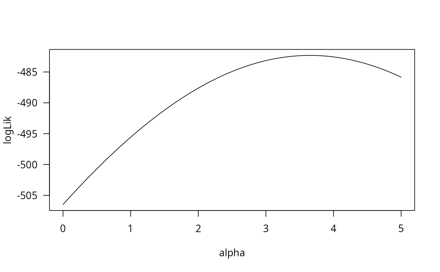 alpha <- optimize(llik, interval = c(0, 5))$minimum
cc_fgls4 <- lm(expenditure ~ age + owner + income + I(income^2), weights = 1/income^alpha,
data = ccard0)
## Table 11.2
cc_fit <- list(cc_ols, cc_wls1, cc_wls2, cc_fgls2, cc_fgls1, cc_fgls3, cc_fgls4)
t(sapply(cc_fit, coef))
#> (Intercept) age owneryes income I(income^2)
#> [1,] -237.12660 -3.086288 27.91120 234.41556 -15.002467
#> [2,] -181.93573 -2.938475 50.47325 202.26384 -12.122090
#> [3,] -114.22064 -2.696285 60.43805 158.52460 -7.258642
#> [4,] -117.99709 -1.229088 50.90827 145.30518 -7.938276
#> [5,] -193.47191 -2.961744 47.30618 209.02210 -12.782103
#> [6,] -130.55515 -2.778092 59.10655 169.88021 -8.614093
#> [7,] -19.30138 -1.705737 58.09942 75.98748 4.392631
t(sapply(cc_fit, function(obj) sqrt(diag(vcov(obj)))))
#> (Intercept) age owneryes income I(income^2)
#> [1,] 199.3244 5.514764 82.91990 80.36466 7.469185
#> [2,] 165.4981 4.603286 69.87638 76.78435 8.273252
#> [3,] 139.6780 3.807233 58.54868 76.39688 9.724617
#> [4,] 101.3706 2.548163 52.81635 46.35491 3.736022
#> [5,] 171.1090 4.764028 72.15562 77.20409 8.082372
#> [6,] 145.0461 3.982370 61.05116 76.18479 9.312051
#> [7,] 117.2006 2.859072 45.10098 84.01104 13.925698
## Table 21.21, Poisson and logit models
cc_pois <- glm(reports ~ age + income + expenditure, data = CreditCard, family = poisson)
summary(cc_pois)
#>
#> Call:
#> glm(formula = reports ~ age + income + expenditure, family = poisson,
#> data = CreditCard)
#>
#> Coefficients:
#> Estimate Std. Error z value Pr(>|z|)
#> (Intercept) -0.819682 0.145272 -5.642 1.68e-08 ***
#> age 0.007181 0.003978 1.805 0.07105 .
#> income 0.077898 0.023940 3.254 0.00114 **
#> expenditure -0.004102 0.000374 -10.968 < 2e-16 ***
#> ---
#> Signif. codes: 0 ‘***’ 0.001 ‘**’ 0.01 ‘*’ 0.05 ‘.’ 0.1 ‘ ’ 1
#>
#> (Dispersion parameter for poisson family taken to be 1)
#>
#> Null deviance: 2347.4 on 1318 degrees of freedom
#> Residual deviance: 2143.9 on 1315 degrees of freedom
#> AIC: 2801.4
#>
#> Number of Fisher Scoring iterations: 7
#>
logLik(cc_pois)
#> 'log Lik.' -1396.719 (df=4)
xhat <- colMeans(CreditCard[, c("age", "income", "expenditure")])
xhat <- as.data.frame(t(xhat))
lambda <- predict(cc_pois, newdata = xhat, type = "response")
ppois(0, lambda) * nrow(CreditCard)
#> [1] 938.597
cc_logit <- glm(factor(reports > 0) ~ age + income + owner,
data = CreditCard, family = binomial)
summary(cc_logit)
#>
#> Call:
#> glm(formula = factor(reports > 0) ~ age + income + owner, family = binomial,
#> data = CreditCard)
#>
#> Coefficients:
#> Estimate Std. Error z value Pr(>|z|)
#> (Intercept) -2.244166 0.251459 -8.925 < 2e-16 ***
#> age 0.022458 0.007313 3.071 0.00213 **
#> income 0.069317 0.041983 1.651 0.09872 .
#> owneryes -0.376620 0.157799 -2.387 0.01700 *
#> ---
#> Signif. codes: 0 ‘***’ 0.001 ‘**’ 0.01 ‘*’ 0.05 ‘.’ 0.1 ‘ ’ 1
#>
#> (Dispersion parameter for binomial family taken to be 1)
#>
#> Null deviance: 1306.6 on 1318 degrees of freedom
#> Residual deviance: 1291.1 on 1315 degrees of freedom
#> AIC: 1299.1
#>
#> Number of Fisher Scoring iterations: 4
#>
logLik(cc_logit)
#> 'log Lik.' -645.5649 (df=4)
## Table 21.21, "split population model"
library("pscl")
cc_zip <- zeroinfl(reports ~ age + income + expenditure | age + income + owner,
data = CreditCard)
summary(cc_zip)
#>
#> Call:
#> zeroinfl(formula = reports ~ age + income + expenditure | age + income +
#> owner, data = CreditCard)
#>
#> Pearson residuals:
#> Min 1Q Median 3Q Max
#> -0.7540 -0.4436 -0.3980 -0.3074 11.2583
#>
#> Count model coefficients (poisson with log link):
#> Estimate Std. Error z value Pr(>|z|)
#> (Intercept) 1.0009818 0.2040577 4.905 9.32e-07 ***
#> age -0.0050726 0.0056934 -0.891 0.373
#> income 0.0133224 0.0325209 0.410 0.682
#> expenditure -0.0023586 0.0003207 -7.354 1.92e-13 ***
#>
#> Zero-inflation model coefficients (binomial with logit link):
#> Estimate Std. Error z value Pr(>|z|)
#> (Intercept) 2.154038 0.304421 7.076 1.49e-12 ***
#> age -0.024685 0.008888 -2.777 0.00548 **
#> income -0.116745 0.051498 -2.267 0.02339 *
#> owneryes 0.386539 0.170840 2.263 0.02366 *
#> ---
#> Signif. codes: 0 '***' 0.001 '**' 0.01 '*' 0.05 '.' 0.1 ' ' 1
#>
#> Number of iterations in BFGS optimization: 17
#> Log-likelihood: -1093 on 8 Df
sum(predict(cc_zip, type = "prob")[,1])
#> [1] 1060.261
###################################
## DEM/GBP exchange rate returns ##
###################################
## data as given by Greene (2003)
data("MarkPound")
mp <- round(MarkPound, digits = 6)
## Figure 11.3 in Greene (2003)
plot(mp)
alpha <- optimize(llik, interval = c(0, 5))$minimum
cc_fgls4 <- lm(expenditure ~ age + owner + income + I(income^2), weights = 1/income^alpha,
data = ccard0)
## Table 11.2
cc_fit <- list(cc_ols, cc_wls1, cc_wls2, cc_fgls2, cc_fgls1, cc_fgls3, cc_fgls4)
t(sapply(cc_fit, coef))
#> (Intercept) age owneryes income I(income^2)
#> [1,] -237.12660 -3.086288 27.91120 234.41556 -15.002467
#> [2,] -181.93573 -2.938475 50.47325 202.26384 -12.122090
#> [3,] -114.22064 -2.696285 60.43805 158.52460 -7.258642
#> [4,] -117.99709 -1.229088 50.90827 145.30518 -7.938276
#> [5,] -193.47191 -2.961744 47.30618 209.02210 -12.782103
#> [6,] -130.55515 -2.778092 59.10655 169.88021 -8.614093
#> [7,] -19.30138 -1.705737 58.09942 75.98748 4.392631
t(sapply(cc_fit, function(obj) sqrt(diag(vcov(obj)))))
#> (Intercept) age owneryes income I(income^2)
#> [1,] 199.3244 5.514764 82.91990 80.36466 7.469185
#> [2,] 165.4981 4.603286 69.87638 76.78435 8.273252
#> [3,] 139.6780 3.807233 58.54868 76.39688 9.724617
#> [4,] 101.3706 2.548163 52.81635 46.35491 3.736022
#> [5,] 171.1090 4.764028 72.15562 77.20409 8.082372
#> [6,] 145.0461 3.982370 61.05116 76.18479 9.312051
#> [7,] 117.2006 2.859072 45.10098 84.01104 13.925698
## Table 21.21, Poisson and logit models
cc_pois <- glm(reports ~ age + income + expenditure, data = CreditCard, family = poisson)
summary(cc_pois)
#>
#> Call:
#> glm(formula = reports ~ age + income + expenditure, family = poisson,
#> data = CreditCard)
#>
#> Coefficients:
#> Estimate Std. Error z value Pr(>|z|)
#> (Intercept) -0.819682 0.145272 -5.642 1.68e-08 ***
#> age 0.007181 0.003978 1.805 0.07105 .
#> income 0.077898 0.023940 3.254 0.00114 **
#> expenditure -0.004102 0.000374 -10.968 < 2e-16 ***
#> ---
#> Signif. codes: 0 ‘***’ 0.001 ‘**’ 0.01 ‘*’ 0.05 ‘.’ 0.1 ‘ ’ 1
#>
#> (Dispersion parameter for poisson family taken to be 1)
#>
#> Null deviance: 2347.4 on 1318 degrees of freedom
#> Residual deviance: 2143.9 on 1315 degrees of freedom
#> AIC: 2801.4
#>
#> Number of Fisher Scoring iterations: 7
#>
logLik(cc_pois)
#> 'log Lik.' -1396.719 (df=4)
xhat <- colMeans(CreditCard[, c("age", "income", "expenditure")])
xhat <- as.data.frame(t(xhat))
lambda <- predict(cc_pois, newdata = xhat, type = "response")
ppois(0, lambda) * nrow(CreditCard)
#> [1] 938.597
cc_logit <- glm(factor(reports > 0) ~ age + income + owner,
data = CreditCard, family = binomial)
summary(cc_logit)
#>
#> Call:
#> glm(formula = factor(reports > 0) ~ age + income + owner, family = binomial,
#> data = CreditCard)
#>
#> Coefficients:
#> Estimate Std. Error z value Pr(>|z|)
#> (Intercept) -2.244166 0.251459 -8.925 < 2e-16 ***
#> age 0.022458 0.007313 3.071 0.00213 **
#> income 0.069317 0.041983 1.651 0.09872 .
#> owneryes -0.376620 0.157799 -2.387 0.01700 *
#> ---
#> Signif. codes: 0 ‘***’ 0.001 ‘**’ 0.01 ‘*’ 0.05 ‘.’ 0.1 ‘ ’ 1
#>
#> (Dispersion parameter for binomial family taken to be 1)
#>
#> Null deviance: 1306.6 on 1318 degrees of freedom
#> Residual deviance: 1291.1 on 1315 degrees of freedom
#> AIC: 1299.1
#>
#> Number of Fisher Scoring iterations: 4
#>
logLik(cc_logit)
#> 'log Lik.' -645.5649 (df=4)
## Table 21.21, "split population model"
library("pscl")
cc_zip <- zeroinfl(reports ~ age + income + expenditure | age + income + owner,
data = CreditCard)
summary(cc_zip)
#>
#> Call:
#> zeroinfl(formula = reports ~ age + income + expenditure | age + income +
#> owner, data = CreditCard)
#>
#> Pearson residuals:
#> Min 1Q Median 3Q Max
#> -0.7540 -0.4436 -0.3980 -0.3074 11.2583
#>
#> Count model coefficients (poisson with log link):
#> Estimate Std. Error z value Pr(>|z|)
#> (Intercept) 1.0009818 0.2040577 4.905 9.32e-07 ***
#> age -0.0050726 0.0056934 -0.891 0.373
#> income 0.0133224 0.0325209 0.410 0.682
#> expenditure -0.0023586 0.0003207 -7.354 1.92e-13 ***
#>
#> Zero-inflation model coefficients (binomial with logit link):
#> Estimate Std. Error z value Pr(>|z|)
#> (Intercept) 2.154038 0.304421 7.076 1.49e-12 ***
#> age -0.024685 0.008888 -2.777 0.00548 **
#> income -0.116745 0.051498 -2.267 0.02339 *
#> owneryes 0.386539 0.170840 2.263 0.02366 *
#> ---
#> Signif. codes: 0 '***' 0.001 '**' 0.01 '*' 0.05 '.' 0.1 ' ' 1
#>
#> Number of iterations in BFGS optimization: 17
#> Log-likelihood: -1093 on 8 Df
sum(predict(cc_zip, type = "prob")[,1])
#> [1] 1060.261
###################################
## DEM/GBP exchange rate returns ##
###################################
## data as given by Greene (2003)
data("MarkPound")
mp <- round(MarkPound, digits = 6)
## Figure 11.3 in Greene (2003)
plot(mp)
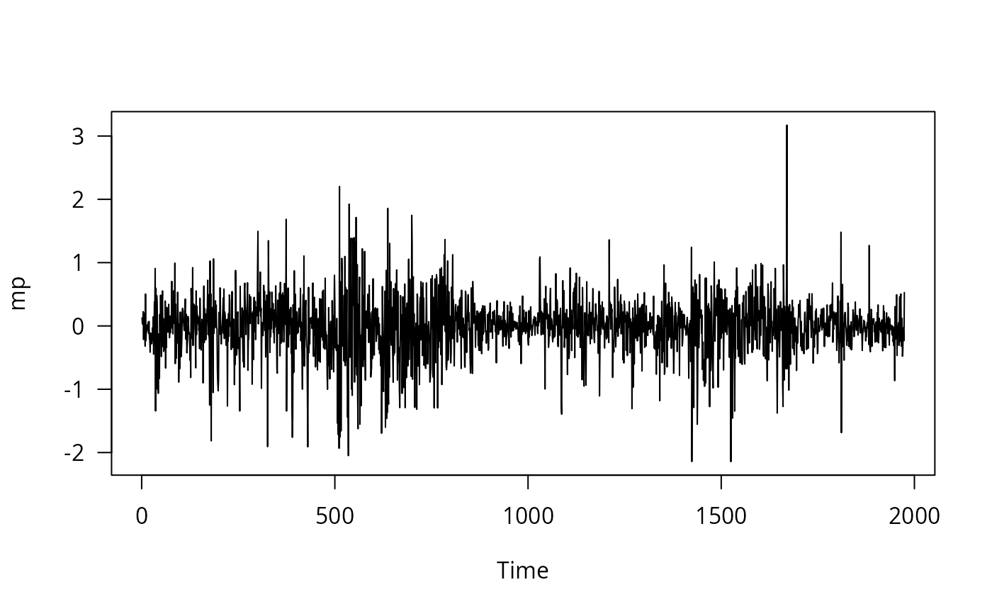 ## Example 11.8 in Greene (2003), Table 11.5
library("tseries")
mp_garch <- garch(mp, grad = "numerical")
#>
#> ***** ESTIMATION WITH NUMERICAL GRADIENT *****
#>
#>
#> I INITIAL X(I) D(I)
#>
#> 1 1.990169e-01 1.000e+00
#> 2 5.000000e-02 1.000e+00
#> 3 5.000000e-02 1.000e+00
#>
#> IT NF F RELDF PRELDF RELDX STPPAR D*STEP NPRELDF
#> 0 1 -5.449e+02
#> 1 3 -5.845e+02 6.78e-02 1.10e-01 2.5e-01 6.4e+03 1.0e-01 3.55e+02
#> 2 5 -5.913e+02 1.15e-02 3.08e-02 7.3e-02 4.6e+00 3.3e-02 4.87e+02
#> 3 6 -5.997e+02 1.40e-02 1.43e-02 7.8e-02 2.0e+00 3.3e-02 9.80e+01
#> 4 7 -6.126e+02 2.11e-02 2.71e-02 1.4e-01 2.0e+00 6.5e-02 6.24e+01
#> 5 8 -6.301e+02 2.77e-02 5.01e-02 1.8e-01 2.0e+00 1.3e-01 3.43e+01
#> 6 9 -6.537e+02 3.61e-02 4.89e-02 2.2e-01 2.0e+00 1.3e-01 1.19e+01
#> 7 11 -6.755e+02 3.24e-02 2.87e-02 1.6e-01 2.0e+00 1.3e-01 1.37e+01
#> 8 13 -6.878e+02 1.78e-02 1.71e-02 9.1e-02 2.0e+00 9.0e-02 2.84e+01
#> 9 16 -6.879e+02 2.73e-04 5.03e-04 1.4e-03 9.8e+00 1.8e-03 2.22e+01
#> 10 17 -6.881e+02 2.59e-04 2.67e-04 1.3e-03 2.1e+00 1.8e-03 1.82e+01
#> 11 18 -6.885e+02 6.02e-04 6.08e-04 2.9e-03 2.0e+00 3.6e-03 1.81e+01
#> 12 22 -6.963e+02 1.12e-02 1.21e-02 6.4e-02 2.0e+00 7.7e-02 1.73e+01
#> 13 26 -6.964e+02 1.07e-04 1.92e-04 5.9e-04 9.1e+00 8.2e-04 8.37e-01
#> 14 27 -6.965e+02 9.85e-05 1.00e-04 5.8e-04 2.4e+00 8.2e-04 6.52e-01
#> 15 28 -6.966e+02 1.80e-04 1.84e-04 1.1e-03 2.0e+00 1.6e-03 6.54e-01
#> 16 33 -7.031e+02 9.26e-03 1.18e-02 7.5e-02 1.9e+00 1.2e-01 6.40e-01
#> 17 35 -7.035e+02 5.47e-04 3.04e-03 1.3e-02 2.0e+00 1.9e-02 3.58e-01
#> 18 36 -7.039e+02 5.98e-04 4.77e-03 1.2e-02 2.0e+00 1.9e-02 1.55e-01
#> 19 37 -7.049e+02 1.45e-03 2.88e-03 1.2e-02 1.7e+00 1.9e-02 3.79e-03
#> 20 38 -7.054e+02 6.23e-04 2.27e-03 1.1e-02 1.7e+00 1.9e-02 1.82e-02
#> 21 39 -7.058e+02 5.69e-04 1.04e-03 1.1e-02 1.3e+00 1.9e-02 2.36e-03
#> 22 41 -7.064e+02 8.39e-04 9.73e-04 2.4e-02 3.0e-01 4.6e-02 1.01e-03
#> 23 42 -7.064e+02 1.88e-05 1.27e-04 4.7e-03 0.0e+00 8.2e-03 1.27e-04
#> 24 43 -7.064e+02 4.80e-05 4.67e-05 1.2e-03 0.0e+00 2.1e-03 4.67e-05
#> 25 44 -7.064e+02 4.71e-07 9.35e-07 7.7e-04 0.0e+00 1.5e-03 9.35e-07
#> 26 45 -7.064e+02 1.82e-07 2.02e-07 1.6e-04 0.0e+00 2.9e-04 2.02e-07
#> 27 46 -7.064e+02 5.22e-09 6.74e-09 4.1e-05 0.0e+00 9.0e-05 6.74e-09
#> 28 47 -7.064e+02 3.70e-10 3.72e-10 1.3e-05 0.0e+00 2.8e-05 3.72e-10
#> 29 48 -7.064e+02 1.97e-13 2.13e-13 1.6e-07 0.0e+00 3.1e-07 2.13e-13
#>
#> ***** RELATIVE FUNCTION CONVERGENCE *****
#>
#> FUNCTION -7.064122e+02 RELDX 1.604e-07
#> FUNC. EVALS 48 GRAD. EVALS 103
#> PRELDF 2.127e-13 NPRELDF 2.127e-13
#>
#> I FINAL X(I) D(I) G(I)
#>
#> 1 1.086690e-02 1.000e+00 9.277e-04
#> 2 1.546040e-01 1.000e+00 4.473e-05
#> 3 8.044204e-01 1.000e+00 9.389e-05
#>
summary(mp_garch)
#>
#> Call:
#> garch(x = mp, grad = "numerical")
#>
#> Model:
#> GARCH(1,1)
#>
#> Residuals:
#> Min 1Q Median 3Q Max
#> -6.797391 -0.537032 -0.002637 0.552328 5.248670
#>
#> Coefficient(s):
#> Estimate Std. Error t value Pr(>|t|)
#> a0 0.010867 0.001297 8.376 <2e-16 ***
#> a1 0.154604 0.013882 11.137 <2e-16 ***
#> b1 0.804420 0.016046 50.133 <2e-16 ***
#> ---
#> Signif. codes: 0 ‘***’ 0.001 ‘**’ 0.01 ‘*’ 0.05 ‘.’ 0.1 ‘ ’ 1
#>
#> Diagnostic Tests:
#> Jarque Bera Test
#>
#> data: Residuals
#> X-squared = 1060, df = 2, p-value < 2.2e-16
#>
#>
#> Box-Ljung test
#>
#> data: Squared.Residuals
#> X-squared = 2.4776, df = 1, p-value = 0.1155
#>
logLik(mp_garch)
#> 'log Lik.' -1106.654 (df=3)
## Greene (2003) also includes a constant and uses different
## standard errors (presumably computed from Hessian), here
## OPG standard errors are used. garchFit() in "fGarch"
## implements the approach used by Greene (2003).
## compare Errata to Greene (2003)
library("dynlm")
res <- residuals(dynlm(mp ~ 1))^2
mp_ols <- dynlm(res ~ L(res, 1:10))
summary(mp_ols)
#>
#> Time series regression with "ts" data:
#> Start = 11, End = 1974
#>
#> Call:
#> dynlm(formula = res ~ L(res, 1:10))
#>
#> Residuals:
#> Min 1Q Median 3Q Max
#> -1.4937 -0.1560 -0.1042 -0.0065 9.7787
#>
#> Coefficients:
#> Estimate Std. Error t value Pr(>|t|)
#> (Intercept) 0.095733 0.014931 6.412 1.80e-10 ***
#> L(res, 1:10)1 0.161696 0.022595 7.156 1.17e-12 ***
#> L(res, 1:10)2 0.094938 0.022882 4.149 3.48e-05 ***
#> L(res, 1:10)3 0.051267 0.022973 2.232 0.0258 *
#> L(res, 1:10)4 0.034278 0.023003 1.490 0.1363
#> L(res, 1:10)5 0.121759 0.023015 5.290 1.36e-07 ***
#> L(res, 1:10)6 -0.007805 0.023015 -0.339 0.7346
#> L(res, 1:10)7 0.003673 0.023003 0.160 0.8731
#> L(res, 1:10)8 0.029509 0.022974 1.284 0.1991
#> L(res, 1:10)9 0.025063 0.022883 1.095 0.2735
#> L(res, 1:10)10 0.054212 0.022595 2.399 0.0165 *
#> ---
#> Signif. codes: 0 ‘***’ 0.001 ‘**’ 0.01 ‘*’ 0.05 ‘.’ 0.1 ‘ ’ 1
#>
#> Residual standard error: 0.5005 on 1953 degrees of freedom
#> Multiple R-squared: 0.09795, Adjusted R-squared: 0.09333
#> F-statistic: 21.21 on 10 and 1953 DF, p-value: < 2.2e-16
#>
logLik(mp_ols)
#> 'log Lik.' -1421.871 (df=12)
summary(mp_ols)$r.squared * length(residuals(mp_ols))
#> [1] 192.3783
################################
## Grunfeld's investment data ##
################################
## subset of data with mistakes
data("Grunfeld", package = "AER")
ggr <- subset(Grunfeld, firm %in% c("General Motors", "US Steel",
"General Electric", "Chrysler", "Westinghouse"))
ggr[c(26, 38), 1] <- c(261.6, 645.2)
ggr[32, 3] <- 232.6
## Tab. 13.4
fm_pool <- lm(invest ~ value + capital, data = ggr)
summary(fm_pool)
#>
#> Call:
#> lm(formula = invest ~ value + capital, data = ggr)
#>
#> Residuals:
#> Min 1Q Median 3Q Max
#> -323.83 -67.52 8.97 41.25 330.66
#>
#> Coefficients:
#> Estimate Std. Error t value Pr(>|t|)
#> (Intercept) -48.02974 21.48017 -2.236 0.0276 *
#> value 0.10509 0.01138 9.236 5.99e-15 ***
#> capital 0.30537 0.04351 7.019 3.06e-10 ***
#> ---
#> Signif. codes: 0 ‘***’ 0.001 ‘**’ 0.01 ‘*’ 0.05 ‘.’ 0.1 ‘ ’ 1
#>
#> Residual standard error: 127.3 on 97 degrees of freedom
#> Multiple R-squared: 0.7789, Adjusted R-squared: 0.7743
#> F-statistic: 170.8 on 2 and 97 DF, p-value: < 2.2e-16
#>
logLik(fm_pool)
#> 'log Lik.' -624.9928 (df=4)
## White correction
sqrt(diag(vcovHC(fm_pool, type = "HC0")))
#> (Intercept) value capital
#> 15.016673443 0.009146375 0.059105263
## heteroskedastic FGLS
auxreg1 <- lm(residuals(fm_pool)^2 ~ firm - 1, data = ggr)
fm_pfgls <- lm(invest ~ value + capital, data = ggr, weights = 1/fitted(auxreg1))
summary(fm_pfgls)
#>
#> Call:
#> lm(formula = invest ~ value + capital, data = ggr, weights = 1/fitted(auxreg1))
#>
#> Weighted Residuals:
#> Min 1Q Median 3Q Max
#> -3.1867 -0.7964 0.0400 0.7323 2.4693
#>
#> Coefficients:
#> Estimate Std. Error t value Pr(>|t|)
#> (Intercept) -36.25370 6.05101 -5.991 3.54e-08 ***
#> value 0.09499 0.00732 12.976 < 2e-16 ***
#> capital 0.33781 0.02986 11.312 < 2e-16 ***
#> ---
#> Signif. codes: 0 ‘***’ 0.001 ‘**’ 0.01 ‘*’ 0.05 ‘.’ 0.1 ‘ ’ 1
#>
#> Residual standard error: 0.988 on 97 degrees of freedom
#> Multiple R-squared: 0.9014, Adjusted R-squared: 0.8993
#> F-statistic: 443.2 on 2 and 97 DF, p-value: < 2.2e-16
#>
## ML, computed as iterated FGLS
sigmasi <- fitted(lm(residuals(fm_pfgls)^2 ~ firm - 1 , data = ggr))
sigmas <- 0
while(any(abs((sigmasi - sigmas)/sigmas) > 1e-7)) {
sigmas <- sigmasi
fm_pfgls_i <- lm(invest ~ value + capital, data = ggr, weights = 1/sigmas)
sigmasi <- fitted(lm(residuals(fm_pfgls_i)^2 ~ firm - 1 , data = ggr))
}
fm_pmlh <- lm(invest ~ value + capital, data = ggr, weights = 1/sigmas)
summary(fm_pmlh)
#>
#> Call:
#> lm(formula = invest ~ value + capital, data = ggr, weights = 1/sigmas)
#>
#> Weighted Residuals:
#> Min 1Q Median 3Q Max
#> -2.5991 -0.8639 -0.3293 0.5610 2.9899
#>
#> Coefficients:
#> Estimate Std. Error t value Pr(>|t|)
#> (Intercept) -23.25818 4.88907 -4.757 6.84e-06 ***
#> value 0.09435 0.00638 14.789 < 2e-16 ***
#> capital 0.33370 0.02238 14.913 < 2e-16 ***
#> ---
#> Signif. codes: 0 ‘***’ 0.001 ‘**’ 0.01 ‘*’ 0.05 ‘.’ 0.1 ‘ ’ 1
#>
#> Residual standard error: 1.015 on 97 degrees of freedom
#> Multiple R-squared: 0.913, Adjusted R-squared: 0.9112
#> F-statistic: 508.7 on 2 and 97 DF, p-value: < 2.2e-16
#>
logLik(fm_pmlh)
#> 'log Lik.' -564.5355 (df=4)
## Tab. 13.5
auxreg2 <- lm(residuals(fm_pfgls)^2 ~ firm - 1, data = ggr)
auxreg3 <- lm(residuals(fm_pmlh)^2 ~ firm - 1, data = ggr)
rbind(
"OLS" = coef(auxreg1),
"Het. FGLS" = coef(auxreg2),
"Het. ML" = coef(auxreg3))
#> firmGeneral Motors firmUS Steel firmGeneral Electric firmChrysler
#> OLS 9410.908 33455.51 34288.49 755.8508
#> Het. FGLS 8612.147 32902.83 36563.24 409.1902
#> Het. ML 8657.885 29824.90 40211.12 175.7844
#> firmWestinghouse
#> OLS 633.4237
#> Het. FGLS 777.9749
#> Het. ML 1241.0107
## Chapter 14: explicitly treat as panel data
library("plm")
pggr <- pdata.frame(ggr, c("firm", "year"))
## Tab. 14.1
library("systemfit")
fm_sur <- systemfit(invest ~ value + capital, data = pggr, method = "SUR",
methodResidCov = "noDfCor")
fm_psur <- systemfit(invest ~ value + capital, data = pggr, method = "SUR", pooled = TRUE,
methodResidCov = "noDfCor", residCovWeighted = TRUE)
## Tab 14.2
fm_ols <- systemfit(invest ~ value + capital, data = pggr, method = "OLS")
fm_pols <- systemfit(invest ~ value + capital, data = pggr, method = "OLS", pooled = TRUE)
## or "by hand"
fm_gm <- lm(invest ~ value + capital, data = ggr, subset = firm == "General Motors")
mean(residuals(fm_gm)^2) ## Greene uses MLE
#> [1] 7160.294
## etc.
fm_pool <- lm(invest ~ value + capital, data = ggr)
## Tab. 14.3 (and Tab 13.4, cross-section ML)
## (not run due to long computation time)
if (FALSE) { # \dontrun{
fm_ml <- systemfit(invest ~ value + capital, data = pggr, method = "SUR",
methodResidCov = "noDfCor", maxiter = 1000, tol = 1e-10)
fm_pml <- systemfit(invest ~ value + capital, data = pggr, method = "SUR", pooled = TRUE,
methodResidCov = "noDfCor", residCovWeighted = TRUE, maxiter = 1000, tol = 1e-10)
} # }
## Fig. 14.2
plot(unlist(residuals(fm_sur)[, c(3, 1, 2, 5, 4)]),
type = "l", ylab = "SUR residuals", ylim = c(-400, 400), xaxs = "i", yaxs = "i")
abline(v = c(20,40,60,80), h = 0, lty = 2)
## Example 11.8 in Greene (2003), Table 11.5
library("tseries")
mp_garch <- garch(mp, grad = "numerical")
#>
#> ***** ESTIMATION WITH NUMERICAL GRADIENT *****
#>
#>
#> I INITIAL X(I) D(I)
#>
#> 1 1.990169e-01 1.000e+00
#> 2 5.000000e-02 1.000e+00
#> 3 5.000000e-02 1.000e+00
#>
#> IT NF F RELDF PRELDF RELDX STPPAR D*STEP NPRELDF
#> 0 1 -5.449e+02
#> 1 3 -5.845e+02 6.78e-02 1.10e-01 2.5e-01 6.4e+03 1.0e-01 3.55e+02
#> 2 5 -5.913e+02 1.15e-02 3.08e-02 7.3e-02 4.6e+00 3.3e-02 4.87e+02
#> 3 6 -5.997e+02 1.40e-02 1.43e-02 7.8e-02 2.0e+00 3.3e-02 9.80e+01
#> 4 7 -6.126e+02 2.11e-02 2.71e-02 1.4e-01 2.0e+00 6.5e-02 6.24e+01
#> 5 8 -6.301e+02 2.77e-02 5.01e-02 1.8e-01 2.0e+00 1.3e-01 3.43e+01
#> 6 9 -6.537e+02 3.61e-02 4.89e-02 2.2e-01 2.0e+00 1.3e-01 1.19e+01
#> 7 11 -6.755e+02 3.24e-02 2.87e-02 1.6e-01 2.0e+00 1.3e-01 1.37e+01
#> 8 13 -6.878e+02 1.78e-02 1.71e-02 9.1e-02 2.0e+00 9.0e-02 2.84e+01
#> 9 16 -6.879e+02 2.73e-04 5.03e-04 1.4e-03 9.8e+00 1.8e-03 2.22e+01
#> 10 17 -6.881e+02 2.59e-04 2.67e-04 1.3e-03 2.1e+00 1.8e-03 1.82e+01
#> 11 18 -6.885e+02 6.02e-04 6.08e-04 2.9e-03 2.0e+00 3.6e-03 1.81e+01
#> 12 22 -6.963e+02 1.12e-02 1.21e-02 6.4e-02 2.0e+00 7.7e-02 1.73e+01
#> 13 26 -6.964e+02 1.07e-04 1.92e-04 5.9e-04 9.1e+00 8.2e-04 8.37e-01
#> 14 27 -6.965e+02 9.85e-05 1.00e-04 5.8e-04 2.4e+00 8.2e-04 6.52e-01
#> 15 28 -6.966e+02 1.80e-04 1.84e-04 1.1e-03 2.0e+00 1.6e-03 6.54e-01
#> 16 33 -7.031e+02 9.26e-03 1.18e-02 7.5e-02 1.9e+00 1.2e-01 6.40e-01
#> 17 35 -7.035e+02 5.47e-04 3.04e-03 1.3e-02 2.0e+00 1.9e-02 3.58e-01
#> 18 36 -7.039e+02 5.98e-04 4.77e-03 1.2e-02 2.0e+00 1.9e-02 1.55e-01
#> 19 37 -7.049e+02 1.45e-03 2.88e-03 1.2e-02 1.7e+00 1.9e-02 3.79e-03
#> 20 38 -7.054e+02 6.23e-04 2.27e-03 1.1e-02 1.7e+00 1.9e-02 1.82e-02
#> 21 39 -7.058e+02 5.69e-04 1.04e-03 1.1e-02 1.3e+00 1.9e-02 2.36e-03
#> 22 41 -7.064e+02 8.39e-04 9.73e-04 2.4e-02 3.0e-01 4.6e-02 1.01e-03
#> 23 42 -7.064e+02 1.88e-05 1.27e-04 4.7e-03 0.0e+00 8.2e-03 1.27e-04
#> 24 43 -7.064e+02 4.80e-05 4.67e-05 1.2e-03 0.0e+00 2.1e-03 4.67e-05
#> 25 44 -7.064e+02 4.71e-07 9.35e-07 7.7e-04 0.0e+00 1.5e-03 9.35e-07
#> 26 45 -7.064e+02 1.82e-07 2.02e-07 1.6e-04 0.0e+00 2.9e-04 2.02e-07
#> 27 46 -7.064e+02 5.22e-09 6.74e-09 4.1e-05 0.0e+00 9.0e-05 6.74e-09
#> 28 47 -7.064e+02 3.70e-10 3.72e-10 1.3e-05 0.0e+00 2.8e-05 3.72e-10
#> 29 48 -7.064e+02 1.97e-13 2.13e-13 1.6e-07 0.0e+00 3.1e-07 2.13e-13
#>
#> ***** RELATIVE FUNCTION CONVERGENCE *****
#>
#> FUNCTION -7.064122e+02 RELDX 1.604e-07
#> FUNC. EVALS 48 GRAD. EVALS 103
#> PRELDF 2.127e-13 NPRELDF 2.127e-13
#>
#> I FINAL X(I) D(I) G(I)
#>
#> 1 1.086690e-02 1.000e+00 9.277e-04
#> 2 1.546040e-01 1.000e+00 4.473e-05
#> 3 8.044204e-01 1.000e+00 9.389e-05
#>
summary(mp_garch)
#>
#> Call:
#> garch(x = mp, grad = "numerical")
#>
#> Model:
#> GARCH(1,1)
#>
#> Residuals:
#> Min 1Q Median 3Q Max
#> -6.797391 -0.537032 -0.002637 0.552328 5.248670
#>
#> Coefficient(s):
#> Estimate Std. Error t value Pr(>|t|)
#> a0 0.010867 0.001297 8.376 <2e-16 ***
#> a1 0.154604 0.013882 11.137 <2e-16 ***
#> b1 0.804420 0.016046 50.133 <2e-16 ***
#> ---
#> Signif. codes: 0 ‘***’ 0.001 ‘**’ 0.01 ‘*’ 0.05 ‘.’ 0.1 ‘ ’ 1
#>
#> Diagnostic Tests:
#> Jarque Bera Test
#>
#> data: Residuals
#> X-squared = 1060, df = 2, p-value < 2.2e-16
#>
#>
#> Box-Ljung test
#>
#> data: Squared.Residuals
#> X-squared = 2.4776, df = 1, p-value = 0.1155
#>
logLik(mp_garch)
#> 'log Lik.' -1106.654 (df=3)
## Greene (2003) also includes a constant and uses different
## standard errors (presumably computed from Hessian), here
## OPG standard errors are used. garchFit() in "fGarch"
## implements the approach used by Greene (2003).
## compare Errata to Greene (2003)
library("dynlm")
res <- residuals(dynlm(mp ~ 1))^2
mp_ols <- dynlm(res ~ L(res, 1:10))
summary(mp_ols)
#>
#> Time series regression with "ts" data:
#> Start = 11, End = 1974
#>
#> Call:
#> dynlm(formula = res ~ L(res, 1:10))
#>
#> Residuals:
#> Min 1Q Median 3Q Max
#> -1.4937 -0.1560 -0.1042 -0.0065 9.7787
#>
#> Coefficients:
#> Estimate Std. Error t value Pr(>|t|)
#> (Intercept) 0.095733 0.014931 6.412 1.80e-10 ***
#> L(res, 1:10)1 0.161696 0.022595 7.156 1.17e-12 ***
#> L(res, 1:10)2 0.094938 0.022882 4.149 3.48e-05 ***
#> L(res, 1:10)3 0.051267 0.022973 2.232 0.0258 *
#> L(res, 1:10)4 0.034278 0.023003 1.490 0.1363
#> L(res, 1:10)5 0.121759 0.023015 5.290 1.36e-07 ***
#> L(res, 1:10)6 -0.007805 0.023015 -0.339 0.7346
#> L(res, 1:10)7 0.003673 0.023003 0.160 0.8731
#> L(res, 1:10)8 0.029509 0.022974 1.284 0.1991
#> L(res, 1:10)9 0.025063 0.022883 1.095 0.2735
#> L(res, 1:10)10 0.054212 0.022595 2.399 0.0165 *
#> ---
#> Signif. codes: 0 ‘***’ 0.001 ‘**’ 0.01 ‘*’ 0.05 ‘.’ 0.1 ‘ ’ 1
#>
#> Residual standard error: 0.5005 on 1953 degrees of freedom
#> Multiple R-squared: 0.09795, Adjusted R-squared: 0.09333
#> F-statistic: 21.21 on 10 and 1953 DF, p-value: < 2.2e-16
#>
logLik(mp_ols)
#> 'log Lik.' -1421.871 (df=12)
summary(mp_ols)$r.squared * length(residuals(mp_ols))
#> [1] 192.3783
################################
## Grunfeld's investment data ##
################################
## subset of data with mistakes
data("Grunfeld", package = "AER")
ggr <- subset(Grunfeld, firm %in% c("General Motors", "US Steel",
"General Electric", "Chrysler", "Westinghouse"))
ggr[c(26, 38), 1] <- c(261.6, 645.2)
ggr[32, 3] <- 232.6
## Tab. 13.4
fm_pool <- lm(invest ~ value + capital, data = ggr)
summary(fm_pool)
#>
#> Call:
#> lm(formula = invest ~ value + capital, data = ggr)
#>
#> Residuals:
#> Min 1Q Median 3Q Max
#> -323.83 -67.52 8.97 41.25 330.66
#>
#> Coefficients:
#> Estimate Std. Error t value Pr(>|t|)
#> (Intercept) -48.02974 21.48017 -2.236 0.0276 *
#> value 0.10509 0.01138 9.236 5.99e-15 ***
#> capital 0.30537 0.04351 7.019 3.06e-10 ***
#> ---
#> Signif. codes: 0 ‘***’ 0.001 ‘**’ 0.01 ‘*’ 0.05 ‘.’ 0.1 ‘ ’ 1
#>
#> Residual standard error: 127.3 on 97 degrees of freedom
#> Multiple R-squared: 0.7789, Adjusted R-squared: 0.7743
#> F-statistic: 170.8 on 2 and 97 DF, p-value: < 2.2e-16
#>
logLik(fm_pool)
#> 'log Lik.' -624.9928 (df=4)
## White correction
sqrt(diag(vcovHC(fm_pool, type = "HC0")))
#> (Intercept) value capital
#> 15.016673443 0.009146375 0.059105263
## heteroskedastic FGLS
auxreg1 <- lm(residuals(fm_pool)^2 ~ firm - 1, data = ggr)
fm_pfgls <- lm(invest ~ value + capital, data = ggr, weights = 1/fitted(auxreg1))
summary(fm_pfgls)
#>
#> Call:
#> lm(formula = invest ~ value + capital, data = ggr, weights = 1/fitted(auxreg1))
#>
#> Weighted Residuals:
#> Min 1Q Median 3Q Max
#> -3.1867 -0.7964 0.0400 0.7323 2.4693
#>
#> Coefficients:
#> Estimate Std. Error t value Pr(>|t|)
#> (Intercept) -36.25370 6.05101 -5.991 3.54e-08 ***
#> value 0.09499 0.00732 12.976 < 2e-16 ***
#> capital 0.33781 0.02986 11.312 < 2e-16 ***
#> ---
#> Signif. codes: 0 ‘***’ 0.001 ‘**’ 0.01 ‘*’ 0.05 ‘.’ 0.1 ‘ ’ 1
#>
#> Residual standard error: 0.988 on 97 degrees of freedom
#> Multiple R-squared: 0.9014, Adjusted R-squared: 0.8993
#> F-statistic: 443.2 on 2 and 97 DF, p-value: < 2.2e-16
#>
## ML, computed as iterated FGLS
sigmasi <- fitted(lm(residuals(fm_pfgls)^2 ~ firm - 1 , data = ggr))
sigmas <- 0
while(any(abs((sigmasi - sigmas)/sigmas) > 1e-7)) {
sigmas <- sigmasi
fm_pfgls_i <- lm(invest ~ value + capital, data = ggr, weights = 1/sigmas)
sigmasi <- fitted(lm(residuals(fm_pfgls_i)^2 ~ firm - 1 , data = ggr))
}
fm_pmlh <- lm(invest ~ value + capital, data = ggr, weights = 1/sigmas)
summary(fm_pmlh)
#>
#> Call:
#> lm(formula = invest ~ value + capital, data = ggr, weights = 1/sigmas)
#>
#> Weighted Residuals:
#> Min 1Q Median 3Q Max
#> -2.5991 -0.8639 -0.3293 0.5610 2.9899
#>
#> Coefficients:
#> Estimate Std. Error t value Pr(>|t|)
#> (Intercept) -23.25818 4.88907 -4.757 6.84e-06 ***
#> value 0.09435 0.00638 14.789 < 2e-16 ***
#> capital 0.33370 0.02238 14.913 < 2e-16 ***
#> ---
#> Signif. codes: 0 ‘***’ 0.001 ‘**’ 0.01 ‘*’ 0.05 ‘.’ 0.1 ‘ ’ 1
#>
#> Residual standard error: 1.015 on 97 degrees of freedom
#> Multiple R-squared: 0.913, Adjusted R-squared: 0.9112
#> F-statistic: 508.7 on 2 and 97 DF, p-value: < 2.2e-16
#>
logLik(fm_pmlh)
#> 'log Lik.' -564.5355 (df=4)
## Tab. 13.5
auxreg2 <- lm(residuals(fm_pfgls)^2 ~ firm - 1, data = ggr)
auxreg3 <- lm(residuals(fm_pmlh)^2 ~ firm - 1, data = ggr)
rbind(
"OLS" = coef(auxreg1),
"Het. FGLS" = coef(auxreg2),
"Het. ML" = coef(auxreg3))
#> firmGeneral Motors firmUS Steel firmGeneral Electric firmChrysler
#> OLS 9410.908 33455.51 34288.49 755.8508
#> Het. FGLS 8612.147 32902.83 36563.24 409.1902
#> Het. ML 8657.885 29824.90 40211.12 175.7844
#> firmWestinghouse
#> OLS 633.4237
#> Het. FGLS 777.9749
#> Het. ML 1241.0107
## Chapter 14: explicitly treat as panel data
library("plm")
pggr <- pdata.frame(ggr, c("firm", "year"))
## Tab. 14.1
library("systemfit")
fm_sur <- systemfit(invest ~ value + capital, data = pggr, method = "SUR",
methodResidCov = "noDfCor")
fm_psur <- systemfit(invest ~ value + capital, data = pggr, method = "SUR", pooled = TRUE,
methodResidCov = "noDfCor", residCovWeighted = TRUE)
## Tab 14.2
fm_ols <- systemfit(invest ~ value + capital, data = pggr, method = "OLS")
fm_pols <- systemfit(invest ~ value + capital, data = pggr, method = "OLS", pooled = TRUE)
## or "by hand"
fm_gm <- lm(invest ~ value + capital, data = ggr, subset = firm == "General Motors")
mean(residuals(fm_gm)^2) ## Greene uses MLE
#> [1] 7160.294
## etc.
fm_pool <- lm(invest ~ value + capital, data = ggr)
## Tab. 14.3 (and Tab 13.4, cross-section ML)
## (not run due to long computation time)
if (FALSE) { # \dontrun{
fm_ml <- systemfit(invest ~ value + capital, data = pggr, method = "SUR",
methodResidCov = "noDfCor", maxiter = 1000, tol = 1e-10)
fm_pml <- systemfit(invest ~ value + capital, data = pggr, method = "SUR", pooled = TRUE,
methodResidCov = "noDfCor", residCovWeighted = TRUE, maxiter = 1000, tol = 1e-10)
} # }
## Fig. 14.2
plot(unlist(residuals(fm_sur)[, c(3, 1, 2, 5, 4)]),
type = "l", ylab = "SUR residuals", ylim = c(-400, 400), xaxs = "i", yaxs = "i")
abline(v = c(20,40,60,80), h = 0, lty = 2)
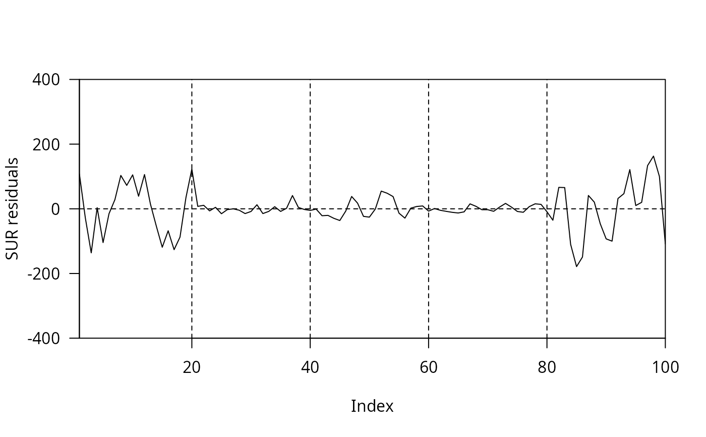 ###################
## Klein model I ##
###################
## data
data("KleinI", package = "AER")
## Tab. 15.3, OLS
library("dynlm")
fm_cons <- dynlm(consumption ~ cprofits + L(cprofits) + I(pwage + gwage), data = KleinI)
fm_inv <- dynlm(invest ~ cprofits + L(cprofits) + capital, data = KleinI)
fm_pwage <- dynlm(pwage ~ gnp + L(gnp) + I(time(gnp) - 1931), data = KleinI)
summary(fm_cons)
#>
#> Time series regression with "ts" data:
#> Start = 1921, End = 1941
#>
#> Call:
#> dynlm(formula = consumption ~ cprofits + L(cprofits) + I(pwage +
#> gwage), data = KleinI)
#>
#> Residuals:
#> Min 1Q Median 3Q Max
#> -2.17345 -0.43597 -0.03466 0.78508 1.61650
#>
#> Coefficients:
#> Estimate Std. Error t value Pr(>|t|)
#> (Intercept) 16.23660 1.30270 12.464 5.62e-10 ***
#> cprofits 0.19293 0.09121 2.115 0.0495 *
#> L(cprofits) 0.08988 0.09065 0.992 0.3353
#> I(pwage + gwage) 0.79622 0.03994 19.933 3.16e-13 ***
#> ---
#> Signif. codes: 0 ‘***’ 0.001 ‘**’ 0.01 ‘*’ 0.05 ‘.’ 0.1 ‘ ’ 1
#>
#> Residual standard error: 1.026 on 17 degrees of freedom
#> Multiple R-squared: 0.981, Adjusted R-squared: 0.9777
#> F-statistic: 292.7 on 3 and 17 DF, p-value: 7.938e-15
#>
summary(fm_inv)
#>
#> Time series regression with "ts" data:
#> Start = 1921, End = 1941
#>
#> Call:
#> dynlm(formula = invest ~ cprofits + L(cprofits) + capital, data = KleinI)
#>
#> Residuals:
#> Min 1Q Median 3Q Max
#> -2.56562 -0.63169 0.03687 0.41542 1.49226
#>
#> Coefficients:
#> Estimate Std. Error t value Pr(>|t|)
#> (Intercept) 10.12579 5.46555 1.853 0.081374 .
#> cprofits 0.47964 0.09711 4.939 0.000125 ***
#> L(cprofits) 0.33304 0.10086 3.302 0.004212 **
#> capital -0.11179 0.02673 -4.183 0.000624 ***
#> ---
#> Signif. codes: 0 ‘***’ 0.001 ‘**’ 0.01 ‘*’ 0.05 ‘.’ 0.1 ‘ ’ 1
#>
#> Residual standard error: 1.009 on 17 degrees of freedom
#> Multiple R-squared: 0.9313, Adjusted R-squared: 0.9192
#> F-statistic: 76.88 on 3 and 17 DF, p-value: 4.299e-10
#>
summary(fm_pwage)
#>
#> Time series regression with "ts" data:
#> Start = 1921, End = 1941
#>
#> Call:
#> dynlm(formula = pwage ~ gnp + L(gnp) + I(time(gnp) - 1931), data = KleinI)
#>
#> Residuals:
#> Min 1Q Median 3Q Max
#> -1.29418 -0.46875 0.01376 0.45027 1.19569
#>
#> Coefficients:
#> Estimate Std. Error t value Pr(>|t|)
#> (Intercept) 1.49704 1.27003 1.179 0.254736
#> gnp 0.43948 0.03241 13.561 1.52e-10 ***
#> L(gnp) 0.14609 0.03742 3.904 0.001142 **
#> I(time(gnp) - 1931) 0.13025 0.03191 4.082 0.000777 ***
#> ---
#> Signif. codes: 0 ‘***’ 0.001 ‘**’ 0.01 ‘*’ 0.05 ‘.’ 0.1 ‘ ’ 1
#>
#> Residual standard error: 0.7671 on 17 degrees of freedom
#> Multiple R-squared: 0.9874, Adjusted R-squared: 0.9852
#> F-statistic: 444.6 on 3 and 17 DF, p-value: 2.411e-16
#>
## Notes:
## - capital refers to previous year's capital stock -> no lag needed!
## - trend used by Greene (p. 381, "time trend measured as years from 1931")
## Maddala uses years since 1919
## preparation of data frame for systemfit
KI <- ts.intersect(KleinI, lag(KleinI, k = -1), dframe = TRUE)
names(KI) <- c(colnames(KleinI), paste("L", colnames(KleinI), sep = ""))
KI$trend <- (1921:1941) - 1931
library("systemfit")
system <- list(
consumption = consumption ~ cprofits + Lcprofits + I(pwage + gwage),
invest = invest ~ cprofits + Lcprofits + capital,
pwage = pwage ~ gnp + Lgnp + trend)
## Tab. 15.3 OLS again
fm_ols <- systemfit(system, method = "OLS", data = KI)
summary(fm_ols)
#>
#> systemfit results
#> method: OLS
#>
#> N DF SSR detRCov OLS-R2 McElroy-R2
#> system 63 51 45.2069 0.37084 0.977268 0.991302
#>
#> N DF SSR MSE RMSE R2 Adj R2
#> consumption 21 17 17.8794 1.051732 1.025540 0.981008 0.977657
#> invest 21 17 17.3227 1.018982 1.009447 0.931348 0.919233
#> pwage 21 17 10.0047 0.588515 0.767147 0.987414 0.985193
#>
#> The covariance matrix of the residuals
#> consumption invest pwage
#> consumption 1.0517323 0.0611432 -0.470419
#> invest 0.0611432 1.0189825 0.149681
#> pwage -0.4704191 0.1496807 0.588515
#>
#> The correlations of the residuals
#> consumption invest pwage
#> consumption 1.0000000 0.0590626 -0.597935
#> invest 0.0590626 1.0000000 0.193288
#> pwage -0.5979346 0.1932875 1.000000
#>
#>
#> OLS estimates for 'consumption' (equation 1)
#> Model Formula: consumption ~ cprofits + Lcprofits + I(pwage + gwage)
#> <environment: 0x5bb5fa905190>
#>
#> Estimate Std. Error t value Pr(>|t|)
#> (Intercept) 16.2366003 1.3026983 12.46382 5.6208e-10 ***
#> cprofits 0.1929344 0.0912102 2.11527 0.049474 *
#> Lcprofits 0.0898849 0.0906479 0.99158 0.335306
#> I(pwage + gwage) 0.7962187 0.0399439 19.93342 3.1619e-13 ***
#> ---
#> Signif. codes: 0 ‘***’ 0.001 ‘**’ 0.01 ‘*’ 0.05 ‘.’ 0.1 ‘ ’ 1
#>
#> Residual standard error: 1.02554 on 17 degrees of freedom
#> Number of observations: 21 Degrees of Freedom: 17
#> SSR: 17.879449 MSE: 1.051732 Root MSE: 1.02554
#> Multiple R-Squared: 0.981008 Adjusted R-Squared: 0.977657
#>
#>
#> OLS estimates for 'invest' (equation 2)
#> Model Formula: invest ~ cprofits + Lcprofits + capital
#> <environment: 0x5bb5fa905190>
#>
#> Estimate Std. Error t value Pr(>|t|)
#> (Intercept) 10.1257885 5.4655465 1.85266 0.08137418 .
#> cprofits 0.4796356 0.0971146 4.93886 0.00012456 ***
#> Lcprofits 0.3330387 0.1008592 3.30202 0.00421173 **
#> capital -0.1117947 0.0267276 -4.18275 0.00062445 ***
#> ---
#> Signif. codes: 0 ‘***’ 0.001 ‘**’ 0.01 ‘*’ 0.05 ‘.’ 0.1 ‘ ’ 1
#>
#> Residual standard error: 1.009447 on 17 degrees of freedom
#> Number of observations: 21 Degrees of Freedom: 17
#> SSR: 17.322702 MSE: 1.018982 Root MSE: 1.009447
#> Multiple R-Squared: 0.931348 Adjusted R-Squared: 0.919233
#>
#>
#> OLS estimates for 'pwage' (equation 3)
#> Model Formula: pwage ~ gnp + Lgnp + trend
#> <environment: 0x5bb5fa905190>
#>
#> Estimate Std. Error t value Pr(>|t|)
#> (Intercept) 1.4970438 1.2700320 1.17874 0.25473559
#> gnp 0.4394770 0.0324076 13.56093 1.5169e-10 ***
#> Lgnp 0.1460899 0.0374231 3.90373 0.00114240 **
#> trend 0.1302452 0.0319103 4.08160 0.00077703 ***
#> ---
#> Signif. codes: 0 ‘***’ 0.001 ‘**’ 0.01 ‘*’ 0.05 ‘.’ 0.1 ‘ ’ 1
#>
#> Residual standard error: 0.767147 on 17 degrees of freedom
#> Number of observations: 21 Degrees of Freedom: 17
#> SSR: 10.00475 MSE: 0.588515 Root MSE: 0.767147
#> Multiple R-Squared: 0.987414 Adjusted R-Squared: 0.985193
#>
## Tab. 15.3 2SLS, 3SLS, I3SLS
inst <- ~ Lcprofits + capital + Lgnp + gexpenditure + taxes + trend + gwage
fm_2sls <- systemfit(system, method = "2SLS", inst = inst,
methodResidCov = "noDfCor", data = KI)
fm_3sls <- systemfit(system, method = "3SLS", inst = inst,
methodResidCov = "noDfCor", data = KI)
fm_i3sls <- systemfit(system, method = "3SLS", inst = inst,
methodResidCov = "noDfCor", maxiter = 100, data = KI)
############################################
## Transportation equipment manufacturing ##
############################################
## data
data("Equipment", package = "AER")
## Example 17.5
## Cobb-Douglas
fm_cd <- lm(log(valueadded/firms) ~ log(capital/firms) + log(labor/firms),
data = Equipment)
## generalized Cobb-Douglas with Zellner-Revankar trafo
GCobbDouglas <- function(theta)
lm(I(log(valueadded/firms) + theta * valueadded/firms) ~ log(capital/firms) + log(labor/firms),
data = Equipment)
## yields classical Cobb-Douglas for theta = 0
fm_cd0 <- GCobbDouglas(0)
## ML estimation of generalized model
## choose starting values from classical model
par0 <- as.vector(c(coef(fm_cd0), 0, mean(residuals(fm_cd0)^2)))
## set up likelihood function
nlogL <- function(par) {
beta <- par[1:3]
theta <- par[4]
sigma2 <- par[5]
Y <- with(Equipment, valueadded/firms)
K <- with(Equipment, capital/firms)
L <- with(Equipment, labor/firms)
rhs <- beta[1] + beta[2] * log(K) + beta[3] * log(L)
lhs <- log(Y) + theta * Y
rval <- sum(log(1 + theta * Y) - log(Y) +
dnorm(lhs, mean = rhs, sd = sqrt(sigma2), log = TRUE))
return(-rval)
}
## optimization
opt <- optim(par0, nlogL, hessian = TRUE)
#> Warning: NaNs produced
#> Warning: NaNs produced
## Table 17.2
opt$par
#> [1] 2.91468783 0.34997794 1.09232479 0.10666219 0.04274876
sqrt(diag(solve(opt$hessian)))[1:4]
#> [1] 0.36055500 0.09671393 0.14079052 0.05849648
-opt$value
#> [1] -8.939045
## re-fit ML model
fm_ml <- GCobbDouglas(opt$par[4])
deviance(fm_ml)
#> [1] 1.068552
sqrt(diag(vcov(fm_ml)))
#> (Intercept) log(capital/firms) log(labor/firms)
#> 0.12533876 0.09435337 0.11497723
## fit NLS model
rss <- function(theta) deviance(GCobbDouglas(theta))
optim(0, rss)
#> Warning: one-dimensional optimization by Nelder-Mead is unreliable:
#> use "Brent" or optimize() directly
#> $par
#> [1] -0.03164062
#>
#> $value
#> [1] 0.765549
#>
#> $counts
#> function gradient
#> 26 NA
#>
#> $convergence
#> [1] 0
#>
#> $message
#> NULL
#>
opt2 <- optimize(rss, c(-1, 1))
fm_nls <- GCobbDouglas(opt2$minimum)
-nlogL(c(coef(fm_nls), opt2$minimum, mean(residuals(fm_nls)^2)))
#> [1] -13.62126
############################
## Municipal expenditures ##
############################
## Table 18.2
data("Municipalities", package = "AER")
summary(Municipalities)
#> municipality year expenditures revenues
#> 114 : 9 1979 :265 Min. :0.01223 Min. :0.006228
#> 115 : 9 1980 :265 1st Qu.:0.01622 1st Qu.:0.011339
#> 120 : 9 1981 :265 Median :0.01796 Median :0.012952
#> 123 : 9 1982 :265 Mean :0.01848 Mean :0.013423
#> 125 : 9 1983 :265 3rd Qu.:0.02014 3rd Qu.:0.014821
#> 126 : 9 1984 :265 Max. :0.03388 Max. :0.029142
#> (Other):2331 (Other):795
#> grants
#> Min. :0.001571
#> 1st Qu.:0.004488
#> Median :0.004978
#> Mean :0.005236
#> 3rd Qu.:0.005539
#> Max. :0.012589
#>
###########################
## Program effectiveness ##
###########################
## Table 21.1, col. "Probit"
data("ProgramEffectiveness", package = "AER")
fm_probit <- glm(grade ~ average + testscore + participation,
data = ProgramEffectiveness, family = binomial(link = "probit"))
summary(fm_probit)
#>
#> Call:
#> glm(formula = grade ~ average + testscore + participation, family = binomial(link = "probit"),
#> data = ProgramEffectiveness)
#>
#> Coefficients:
#> Estimate Std. Error z value Pr(>|z|)
#> (Intercept) -7.45231 2.57152 -2.898 0.00376 **
#> average 1.62581 0.68973 2.357 0.01841 *
#> testscore 0.05173 0.08119 0.637 0.52406
#> participationyes 1.42633 0.58695 2.430 0.01510 *
#> ---
#> Signif. codes: 0 ‘***’ 0.001 ‘**’ 0.01 ‘*’ 0.05 ‘.’ 0.1 ‘ ’ 1
#>
#> (Dispersion parameter for binomial family taken to be 1)
#>
#> Null deviance: 41.183 on 31 degrees of freedom
#> Residual deviance: 25.638 on 28 degrees of freedom
#> AIC: 33.638
#>
#> Number of Fisher Scoring iterations: 6
#>
####################################
## Labor force participation data ##
####################################
## data and transformations
data("PSID1976", package = "AER")
PSID1976$kids <- with(PSID1976, factor((youngkids + oldkids) > 0,
levels = c(FALSE, TRUE), labels = c("no", "yes")))
PSID1976$nwincome <- with(PSID1976, (fincome - hours * wage)/1000)
## Example 4.1, Table 4.2
## (reproduced in Example 7.1, Table 7.1)
gr_lm <- lm(log(hours * wage) ~ age + I(age^2) + education + kids,
data = PSID1976, subset = participation == "yes")
summary(gr_lm)
#>
#> Call:
#> lm(formula = log(hours * wage) ~ age + I(age^2) + education +
#> kids, data = PSID1976, subset = participation == "yes")
#>
#> Residuals:
#> Min 1Q Median 3Q Max
#> -4.5305 -0.5266 0.3003 0.8474 1.7568
#>
#> Coefficients:
#> Estimate Std. Error t value Pr(>|t|)
#> (Intercept) 3.2400965 1.7674296 1.833 0.06747 .
#> age 0.2005573 0.0838603 2.392 0.01721 *
#> I(age^2) -0.0023147 0.0009869 -2.345 0.01947 *
#> education 0.0674727 0.0252486 2.672 0.00782 **
#> kidsyes -0.3511952 0.1475326 -2.380 0.01773 *
#> ---
#> Signif. codes: 0 ‘***’ 0.001 ‘**’ 0.01 ‘*’ 0.05 ‘.’ 0.1 ‘ ’ 1
#>
#> Residual standard error: 1.19 on 423 degrees of freedom
#> Multiple R-squared: 0.041, Adjusted R-squared: 0.03193
#> F-statistic: 4.521 on 4 and 423 DF, p-value: 0.001382
#>
vcov(gr_lm)
#> (Intercept) age I(age^2) education kidsyes
#> (Intercept) 3.12380756 -1.440901e-01 1.661740e-03 -9.260920e-03 2.674867e-02
#> age -0.14409007 7.032544e-03 -8.232369e-05 5.085495e-05 -2.641203e-03
#> I(age^2) 0.00166174 -8.232369e-05 9.739279e-07 -4.976114e-07 3.841018e-05
#> education -0.00926092 5.085495e-05 -4.976114e-07 6.374903e-04 -5.461931e-05
#> kidsyes 0.02674867 -2.641203e-03 3.841018e-05 -5.461931e-05 2.176587e-02
## Example 4.5
summary(gr_lm)
#>
#> Call:
#> lm(formula = log(hours * wage) ~ age + I(age^2) + education +
#> kids, data = PSID1976, subset = participation == "yes")
#>
#> Residuals:
#> Min 1Q Median 3Q Max
#> -4.5305 -0.5266 0.3003 0.8474 1.7568
#>
#> Coefficients:
#> Estimate Std. Error t value Pr(>|t|)
#> (Intercept) 3.2400965 1.7674296 1.833 0.06747 .
#> age 0.2005573 0.0838603 2.392 0.01721 *
#> I(age^2) -0.0023147 0.0009869 -2.345 0.01947 *
#> education 0.0674727 0.0252486 2.672 0.00782 **
#> kidsyes -0.3511952 0.1475326 -2.380 0.01773 *
#> ---
#> Signif. codes: 0 ‘***’ 0.001 ‘**’ 0.01 ‘*’ 0.05 ‘.’ 0.1 ‘ ’ 1
#>
#> Residual standard error: 1.19 on 423 degrees of freedom
#> Multiple R-squared: 0.041, Adjusted R-squared: 0.03193
#> F-statistic: 4.521 on 4 and 423 DF, p-value: 0.001382
#>
## or equivalently
gr_lm1 <- lm(log(hours * wage) ~ 1, data = PSID1976, subset = participation == "yes")
anova(gr_lm1, gr_lm)
#> Analysis of Variance Table
#>
#> Model 1: log(hours * wage) ~ 1
#> Model 2: log(hours * wage) ~ age + I(age^2) + education + kids
#> Res.Df RSS Df Sum of Sq F Pr(>F)
#> 1 427 625.08
#> 2 423 599.46 4 25.625 4.5206 0.001382 **
#> ---
#> Signif. codes: 0 ‘***’ 0.001 ‘**’ 0.01 ‘*’ 0.05 ‘.’ 0.1 ‘ ’ 1
## Example 21.4, p. 681, and Tab. 21.3, p. 682
gr_probit1 <- glm(participation ~ age + I(age^2) + I(fincome/10000) + education + kids,
data = PSID1976, family = binomial(link = "probit") )
gr_probit2 <- glm(participation ~ age + I(age^2) + I(fincome/10000) + education,
data = PSID1976, family = binomial(link = "probit"))
gr_probit3 <- glm(participation ~ kids/(age + I(age^2) + I(fincome/10000) + education),
data = PSID1976, family = binomial(link = "probit"))
## LR test of all coefficients
lrtest(gr_probit1)
#> Likelihood ratio test
#>
#> Model 1: participation ~ age + I(age^2) + I(fincome/10000) + education +
#> kids
#> Model 2: participation ~ 1
#> #Df LogLik Df Chisq Pr(>Chisq)
#> 1 6 -490.85
#> 2 1 -514.87 -5 48.051 3.468e-09 ***
#> ---
#> Signif. codes: 0 ‘***’ 0.001 ‘**’ 0.01 ‘*’ 0.05 ‘.’ 0.1 ‘ ’ 1
## Chow-type test
lrtest(gr_probit2, gr_probit3)
#> Likelihood ratio test
#>
#> Model 1: participation ~ age + I(age^2) + I(fincome/10000) + education
#> Model 2: participation ~ kids/(age + I(age^2) + I(fincome/10000) + education)
#> #Df LogLik Df Chisq Pr(>Chisq)
#> 1 5 -496.87
#> 2 10 -489.48 5 14.774 0.01137 *
#> ---
#> Signif. codes: 0 ‘***’ 0.001 ‘**’ 0.01 ‘*’ 0.05 ‘.’ 0.1 ‘ ’ 1
## equivalently:
anova(gr_probit2, gr_probit3, test = "Chisq")
#> Analysis of Deviance Table
#>
#> Model 1: participation ~ age + I(age^2) + I(fincome/10000) + education
#> Model 2: participation ~ kids/(age + I(age^2) + I(fincome/10000) + education)
#> Resid. Df Resid. Dev Df Deviance Pr(>Chi)
#> 1 748 993.73
#> 2 743 978.96 5 14.774 0.01137 *
#> ---
#> Signif. codes: 0 ‘***’ 0.001 ‘**’ 0.01 ‘*’ 0.05 ‘.’ 0.1 ‘ ’ 1
## Table 21.3
summary(gr_probit1)
#>
#> Call:
#> glm(formula = participation ~ age + I(age^2) + I(fincome/10000) +
#> education + kids, family = binomial(link = "probit"), data = PSID1976)
#>
#> Coefficients:
#> Estimate Std. Error z value Pr(>|z|)
#> (Intercept) -4.1568189 1.4040095 -2.961 0.003070 **
#> age 0.1853957 0.0662076 2.800 0.005107 **
#> I(age^2) -0.0024259 0.0007762 -3.125 0.001775 **
#> I(fincome/10000) 0.0458029 0.0430557 1.064 0.287417
#> education 0.0981824 0.0228932 4.289 1.8e-05 ***
#> kidsyes -0.4489872 0.1300252 -3.453 0.000554 ***
#> ---
#> Signif. codes: 0 ‘***’ 0.001 ‘**’ 0.01 ‘*’ 0.05 ‘.’ 0.1 ‘ ’ 1
#>
#> (Dispersion parameter for binomial family taken to be 1)
#>
#> Null deviance: 1029.7 on 752 degrees of freedom
#> Residual deviance: 981.7 on 747 degrees of freedom
#> AIC: 993.7
#>
#> Number of Fisher Scoring iterations: 4
#>
## Example 22.8, Table 22.7, p. 786
library("sampleSelection")
#> Loading required package: maxLik
#> Loading required package: miscTools
#>
#> Please cite the 'maxLik' package as:
#> Henningsen, Arne and Toomet, Ott (2011). maxLik: A package for maximum likelihood estimation in R. Computational Statistics 26(3), 443-458. DOI 10.1007/s00180-010-0217-1.
#>
#> If you have questions, suggestions, or comments regarding the 'maxLik' package, please use a forum or 'tracker' at maxLik's R-Forge site:
#> https://r-forge.r-project.org/projects/maxlik/
gr_2step <- selection(participation ~ age + I(age^2) + fincome + education + kids,
wage ~ experience + I(experience^2) + education + city,
data = PSID1976, method = "2step")
gr_ml <- selection(participation ~ age + I(age^2) + fincome + education + kids,
wage ~ experience + I(experience^2) + education + city,
data = PSID1976, method = "ml")
gr_ols <- lm(wage ~ experience + I(experience^2) + education + city,
data = PSID1976, subset = participation == "yes")
## NOTE: ML estimates agree with Greene, 5e errata.
## Standard errors are based on the Hessian (here), while Greene has BHHH/OPG.
####################
## Ship accidents ##
####################
## subset data
data("ShipAccidents", package = "AER")
sa <- subset(ShipAccidents, service > 0)
## Table 21.20
sa_full <- glm(incidents ~ type + construction + operation, family = poisson,
data = sa, offset = log(service))
summary(sa_full)
#>
#> Call:
#> glm(formula = incidents ~ type + construction + operation, family = poisson,
#> data = sa, offset = log(service))
#>
#> Coefficients:
#> Estimate Std. Error z value Pr(>|z|)
#> (Intercept) -6.40288 0.21752 -29.435 < 2e-16 ***
#> typeB -0.54471 0.17761 -3.067 0.00216 **
#> typeC -0.68876 0.32903 -2.093 0.03632 *
#> typeD -0.07431 0.29056 -0.256 0.79815
#> typeE 0.32053 0.23575 1.360 0.17396
#> construction1965-69 0.69585 0.14966 4.650 3.33e-06 ***
#> construction1970-74 0.81746 0.16984 4.813 1.49e-06 ***
#> construction1975-79 0.44497 0.23324 1.908 0.05642 .
#> operation1975-79 0.38386 0.11826 3.246 0.00117 **
#> ---
#> Signif. codes: 0 ‘***’ 0.001 ‘**’ 0.01 ‘*’ 0.05 ‘.’ 0.1 ‘ ’ 1
#>
#> (Dispersion parameter for poisson family taken to be 1)
#>
#> Null deviance: 146.328 on 33 degrees of freedom
#> Residual deviance: 38.963 on 25 degrees of freedom
#> AIC: 154.83
#>
#> Number of Fisher Scoring iterations: 5
#>
sa_notype <- glm(incidents ~ construction + operation, family = poisson,
data = sa, offset = log(service))
summary(sa_notype)
#>
#> Call:
#> glm(formula = incidents ~ construction + operation, family = poisson,
#> data = sa, offset = log(service))
#>
#> Coefficients:
#> Estimate Std. Error z value Pr(>|z|)
#> (Intercept) -6.9470 0.1269 -54.725 < 2e-16 ***
#> construction1965-69 0.7536 0.1488 5.066 4.07e-07 ***
#> construction1970-74 1.0503 0.1576 6.666 2.63e-11 ***
#> construction1975-79 0.6999 0.2203 3.177 0.00149 **
#> operation1975-79 0.3872 0.1181 3.279 0.00104 **
#> ---
#> Signif. codes: 0 ‘***’ 0.001 ‘**’ 0.01 ‘*’ 0.05 ‘.’ 0.1 ‘ ’ 1
#>
#> (Dispersion parameter for poisson family taken to be 1)
#>
#> Null deviance: 146.328 on 33 degrees of freedom
#> Residual deviance: 62.536 on 29 degrees of freedom
#> AIC: 170.4
#>
#> Number of Fisher Scoring iterations: 4
#>
sa_noperiod <- glm(incidents ~ type + operation, family = poisson,
data = sa, offset = log(service))
summary(sa_noperiod)
#>
#> Call:
#> glm(formula = incidents ~ type + operation, family = poisson,
#> data = sa, offset = log(service))
#>
#> Coefficients:
#> Estimate Std. Error z value Pr(>|z|)
#> (Intercept) -5.8000 0.1784 -32.508 < 2e-16 ***
#> typeB -0.7437 0.1691 -4.397 1.10e-05 ***
#> typeC -0.7549 0.3276 -2.304 0.0212 *
#> typeD -0.1843 0.2876 -0.641 0.5215
#> typeE 0.3842 0.2348 1.636 0.1018
#> operation1975-79 0.5001 0.1116 4.483 7.37e-06 ***
#> ---
#> Signif. codes: 0 ‘***’ 0.001 ‘**’ 0.01 ‘*’ 0.05 ‘.’ 0.1 ‘ ’ 1
#>
#> (Dispersion parameter for poisson family taken to be 1)
#>
#> Null deviance: 146.328 on 33 degrees of freedom
#> Residual deviance: 70.364 on 28 degrees of freedom
#> AIC: 180.23
#>
#> Number of Fisher Scoring iterations: 5
#>
## model comparison
anova(sa_full, sa_notype, test = "Chisq")
#> Analysis of Deviance Table
#>
#> Model 1: incidents ~ type + construction + operation
#> Model 2: incidents ~ construction + operation
#> Resid. Df Resid. Dev Df Deviance Pr(>Chi)
#> 1 25 38.963
#> 2 29 62.536 -4 -23.573 9.725e-05 ***
#> ---
#> Signif. codes: 0 ‘***’ 0.001 ‘**’ 0.01 ‘*’ 0.05 ‘.’ 0.1 ‘ ’ 1
anova(sa_full, sa_noperiod, test = "Chisq")
#> Analysis of Deviance Table
#>
#> Model 1: incidents ~ type + construction + operation
#> Model 2: incidents ~ type + operation
#> Resid. Df Resid. Dev Df Deviance Pr(>Chi)
#> 1 25 38.963
#> 2 28 70.364 -3 -31.401 6.998e-07 ***
#> ---
#> Signif. codes: 0 ‘***’ 0.001 ‘**’ 0.01 ‘*’ 0.05 ‘.’ 0.1 ‘ ’ 1
## test for overdispersion
dispersiontest(sa_full)
#>
#> Overdispersion test
#>
#> data: sa_full
#> z = 0.93429, p-value = 0.1751
#> alternative hypothesis: true dispersion is greater than 1
#> sample estimates:
#> dispersion
#> 1.317918
#>
dispersiontest(sa_full, trafo = 2)
#>
#> Overdispersion test
#>
#> data: sa_full
#> z = -0.6129, p-value = 0.73
#> alternative hypothesis: true alpha is greater than 0
#> sample estimates:
#> alpha
#> -0.0111868
#>
######################################
## Fair's extramarital affairs data ##
######################################
## data
data("Affairs", package = "AER")
## Tab. 22.3 and 22.4
fm_ols <- lm(affairs ~ age + yearsmarried + religiousness + occupation + rating,
data = Affairs)
fm_probit <- glm(I(affairs > 0) ~ age + yearsmarried + religiousness + occupation + rating,
data = Affairs, family = binomial(link = "probit"))
fm_tobit <- tobit(affairs ~ age + yearsmarried + religiousness + occupation + rating,
data = Affairs)
fm_tobit2 <- tobit(affairs ~ age + yearsmarried + religiousness + occupation + rating,
right = 4, data = Affairs)
fm_pois <- glm(affairs ~ age + yearsmarried + religiousness + occupation + rating,
data = Affairs, family = poisson)
library("MASS")
fm_nb <- glm.nb(affairs ~ age + yearsmarried + religiousness + occupation + rating,
data = Affairs)
## Tab. 22.6
library("pscl")
fm_zip <- zeroinfl(affairs ~ age + yearsmarried + religiousness + occupation + rating | age +
yearsmarried + religiousness + occupation + rating, data = Affairs)
######################
## Strike durations ##
######################
## data and package
data("StrikeDuration", package = "AER")
library("MASS")
## Table 22.10
fit_exp <- fitdistr(StrikeDuration$duration, "exponential")
fit_wei <- fitdistr(StrikeDuration$duration, "weibull")
fit_wei$estimate[2]^(-1)
#> scale
#> 0.02432637
fit_lnorm <- fitdistr(StrikeDuration$duration, "lognormal")
1/fit_lnorm$estimate[2]
#> sdlog
#> 0.7787838
exp(-fit_lnorm$estimate[1])
#> meanlog
#> 0.0448489
## Weibull and lognormal distribution have
## different parameterizations, see Greene p. 794
## Example 22.10
library("survival")
fm_wei <- survreg(Surv(duration) ~ uoutput, dist = "weibull", data = StrikeDuration)
summary(fm_wei)
#>
#> Call:
#> survreg(formula = Surv(duration) ~ uoutput, data = StrikeDuration,
#> dist = "weibull")
#> Value Std. Error z p
#> (Intercept) 3.77977 0.13670 27.65 <2e-16
#> uoutput -9.33220 2.93756 -3.18 0.0015
#> Log(scale) -0.00783 0.10050 -0.08 0.9379
#>
#> Scale= 0.992
#>
#> Weibull distribution
#> Loglik(model)= -289.8 Loglik(intercept only)= -294.4
#> Chisq= 9.28 on 1 degrees of freedom, p= 0.0023
#> Number of Newton-Raphson Iterations: 6
#> n= 62
#>
# }
###################
## Klein model I ##
###################
## data
data("KleinI", package = "AER")
## Tab. 15.3, OLS
library("dynlm")
fm_cons <- dynlm(consumption ~ cprofits + L(cprofits) + I(pwage + gwage), data = KleinI)
fm_inv <- dynlm(invest ~ cprofits + L(cprofits) + capital, data = KleinI)
fm_pwage <- dynlm(pwage ~ gnp + L(gnp) + I(time(gnp) - 1931), data = KleinI)
summary(fm_cons)
#>
#> Time series regression with "ts" data:
#> Start = 1921, End = 1941
#>
#> Call:
#> dynlm(formula = consumption ~ cprofits + L(cprofits) + I(pwage +
#> gwage), data = KleinI)
#>
#> Residuals:
#> Min 1Q Median 3Q Max
#> -2.17345 -0.43597 -0.03466 0.78508 1.61650
#>
#> Coefficients:
#> Estimate Std. Error t value Pr(>|t|)
#> (Intercept) 16.23660 1.30270 12.464 5.62e-10 ***
#> cprofits 0.19293 0.09121 2.115 0.0495 *
#> L(cprofits) 0.08988 0.09065 0.992 0.3353
#> I(pwage + gwage) 0.79622 0.03994 19.933 3.16e-13 ***
#> ---
#> Signif. codes: 0 ‘***’ 0.001 ‘**’ 0.01 ‘*’ 0.05 ‘.’ 0.1 ‘ ’ 1
#>
#> Residual standard error: 1.026 on 17 degrees of freedom
#> Multiple R-squared: 0.981, Adjusted R-squared: 0.9777
#> F-statistic: 292.7 on 3 and 17 DF, p-value: 7.938e-15
#>
summary(fm_inv)
#>
#> Time series regression with "ts" data:
#> Start = 1921, End = 1941
#>
#> Call:
#> dynlm(formula = invest ~ cprofits + L(cprofits) + capital, data = KleinI)
#>
#> Residuals:
#> Min 1Q Median 3Q Max
#> -2.56562 -0.63169 0.03687 0.41542 1.49226
#>
#> Coefficients:
#> Estimate Std. Error t value Pr(>|t|)
#> (Intercept) 10.12579 5.46555 1.853 0.081374 .
#> cprofits 0.47964 0.09711 4.939 0.000125 ***
#> L(cprofits) 0.33304 0.10086 3.302 0.004212 **
#> capital -0.11179 0.02673 -4.183 0.000624 ***
#> ---
#> Signif. codes: 0 ‘***’ 0.001 ‘**’ 0.01 ‘*’ 0.05 ‘.’ 0.1 ‘ ’ 1
#>
#> Residual standard error: 1.009 on 17 degrees of freedom
#> Multiple R-squared: 0.9313, Adjusted R-squared: 0.9192
#> F-statistic: 76.88 on 3 and 17 DF, p-value: 4.299e-10
#>
summary(fm_pwage)
#>
#> Time series regression with "ts" data:
#> Start = 1921, End = 1941
#>
#> Call:
#> dynlm(formula = pwage ~ gnp + L(gnp) + I(time(gnp) - 1931), data = KleinI)
#>
#> Residuals:
#> Min 1Q Median 3Q Max
#> -1.29418 -0.46875 0.01376 0.45027 1.19569
#>
#> Coefficients:
#> Estimate Std. Error t value Pr(>|t|)
#> (Intercept) 1.49704 1.27003 1.179 0.254736
#> gnp 0.43948 0.03241 13.561 1.52e-10 ***
#> L(gnp) 0.14609 0.03742 3.904 0.001142 **
#> I(time(gnp) - 1931) 0.13025 0.03191 4.082 0.000777 ***
#> ---
#> Signif. codes: 0 ‘***’ 0.001 ‘**’ 0.01 ‘*’ 0.05 ‘.’ 0.1 ‘ ’ 1
#>
#> Residual standard error: 0.7671 on 17 degrees of freedom
#> Multiple R-squared: 0.9874, Adjusted R-squared: 0.9852
#> F-statistic: 444.6 on 3 and 17 DF, p-value: 2.411e-16
#>
## Notes:
## - capital refers to previous year's capital stock -> no lag needed!
## - trend used by Greene (p. 381, "time trend measured as years from 1931")
## Maddala uses years since 1919
## preparation of data frame for systemfit
KI <- ts.intersect(KleinI, lag(KleinI, k = -1), dframe = TRUE)
names(KI) <- c(colnames(KleinI), paste("L", colnames(KleinI), sep = ""))
KI$trend <- (1921:1941) - 1931
library("systemfit")
system <- list(
consumption = consumption ~ cprofits + Lcprofits + I(pwage + gwage),
invest = invest ~ cprofits + Lcprofits + capital,
pwage = pwage ~ gnp + Lgnp + trend)
## Tab. 15.3 OLS again
fm_ols <- systemfit(system, method = "OLS", data = KI)
summary(fm_ols)
#>
#> systemfit results
#> method: OLS
#>
#> N DF SSR detRCov OLS-R2 McElroy-R2
#> system 63 51 45.2069 0.37084 0.977268 0.991302
#>
#> N DF SSR MSE RMSE R2 Adj R2
#> consumption 21 17 17.8794 1.051732 1.025540 0.981008 0.977657
#> invest 21 17 17.3227 1.018982 1.009447 0.931348 0.919233
#> pwage 21 17 10.0047 0.588515 0.767147 0.987414 0.985193
#>
#> The covariance matrix of the residuals
#> consumption invest pwage
#> consumption 1.0517323 0.0611432 -0.470419
#> invest 0.0611432 1.0189825 0.149681
#> pwage -0.4704191 0.1496807 0.588515
#>
#> The correlations of the residuals
#> consumption invest pwage
#> consumption 1.0000000 0.0590626 -0.597935
#> invest 0.0590626 1.0000000 0.193288
#> pwage -0.5979346 0.1932875 1.000000
#>
#>
#> OLS estimates for 'consumption' (equation 1)
#> Model Formula: consumption ~ cprofits + Lcprofits + I(pwage + gwage)
#> <environment: 0x5bb5fa905190>
#>
#> Estimate Std. Error t value Pr(>|t|)
#> (Intercept) 16.2366003 1.3026983 12.46382 5.6208e-10 ***
#> cprofits 0.1929344 0.0912102 2.11527 0.049474 *
#> Lcprofits 0.0898849 0.0906479 0.99158 0.335306
#> I(pwage + gwage) 0.7962187 0.0399439 19.93342 3.1619e-13 ***
#> ---
#> Signif. codes: 0 ‘***’ 0.001 ‘**’ 0.01 ‘*’ 0.05 ‘.’ 0.1 ‘ ’ 1
#>
#> Residual standard error: 1.02554 on 17 degrees of freedom
#> Number of observations: 21 Degrees of Freedom: 17
#> SSR: 17.879449 MSE: 1.051732 Root MSE: 1.02554
#> Multiple R-Squared: 0.981008 Adjusted R-Squared: 0.977657
#>
#>
#> OLS estimates for 'invest' (equation 2)
#> Model Formula: invest ~ cprofits + Lcprofits + capital
#> <environment: 0x5bb5fa905190>
#>
#> Estimate Std. Error t value Pr(>|t|)
#> (Intercept) 10.1257885 5.4655465 1.85266 0.08137418 .
#> cprofits 0.4796356 0.0971146 4.93886 0.00012456 ***
#> Lcprofits 0.3330387 0.1008592 3.30202 0.00421173 **
#> capital -0.1117947 0.0267276 -4.18275 0.00062445 ***
#> ---
#> Signif. codes: 0 ‘***’ 0.001 ‘**’ 0.01 ‘*’ 0.05 ‘.’ 0.1 ‘ ’ 1
#>
#> Residual standard error: 1.009447 on 17 degrees of freedom
#> Number of observations: 21 Degrees of Freedom: 17
#> SSR: 17.322702 MSE: 1.018982 Root MSE: 1.009447
#> Multiple R-Squared: 0.931348 Adjusted R-Squared: 0.919233
#>
#>
#> OLS estimates for 'pwage' (equation 3)
#> Model Formula: pwage ~ gnp + Lgnp + trend
#> <environment: 0x5bb5fa905190>
#>
#> Estimate Std. Error t value Pr(>|t|)
#> (Intercept) 1.4970438 1.2700320 1.17874 0.25473559
#> gnp 0.4394770 0.0324076 13.56093 1.5169e-10 ***
#> Lgnp 0.1460899 0.0374231 3.90373 0.00114240 **
#> trend 0.1302452 0.0319103 4.08160 0.00077703 ***
#> ---
#> Signif. codes: 0 ‘***’ 0.001 ‘**’ 0.01 ‘*’ 0.05 ‘.’ 0.1 ‘ ’ 1
#>
#> Residual standard error: 0.767147 on 17 degrees of freedom
#> Number of observations: 21 Degrees of Freedom: 17
#> SSR: 10.00475 MSE: 0.588515 Root MSE: 0.767147
#> Multiple R-Squared: 0.987414 Adjusted R-Squared: 0.985193
#>
## Tab. 15.3 2SLS, 3SLS, I3SLS
inst <- ~ Lcprofits + capital + Lgnp + gexpenditure + taxes + trend + gwage
fm_2sls <- systemfit(system, method = "2SLS", inst = inst,
methodResidCov = "noDfCor", data = KI)
fm_3sls <- systemfit(system, method = "3SLS", inst = inst,
methodResidCov = "noDfCor", data = KI)
fm_i3sls <- systemfit(system, method = "3SLS", inst = inst,
methodResidCov = "noDfCor", maxiter = 100, data = KI)
############################################
## Transportation equipment manufacturing ##
############################################
## data
data("Equipment", package = "AER")
## Example 17.5
## Cobb-Douglas
fm_cd <- lm(log(valueadded/firms) ~ log(capital/firms) + log(labor/firms),
data = Equipment)
## generalized Cobb-Douglas with Zellner-Revankar trafo
GCobbDouglas <- function(theta)
lm(I(log(valueadded/firms) + theta * valueadded/firms) ~ log(capital/firms) + log(labor/firms),
data = Equipment)
## yields classical Cobb-Douglas for theta = 0
fm_cd0 <- GCobbDouglas(0)
## ML estimation of generalized model
## choose starting values from classical model
par0 <- as.vector(c(coef(fm_cd0), 0, mean(residuals(fm_cd0)^2)))
## set up likelihood function
nlogL <- function(par) {
beta <- par[1:3]
theta <- par[4]
sigma2 <- par[5]
Y <- with(Equipment, valueadded/firms)
K <- with(Equipment, capital/firms)
L <- with(Equipment, labor/firms)
rhs <- beta[1] + beta[2] * log(K) + beta[3] * log(L)
lhs <- log(Y) + theta * Y
rval <- sum(log(1 + theta * Y) - log(Y) +
dnorm(lhs, mean = rhs, sd = sqrt(sigma2), log = TRUE))
return(-rval)
}
## optimization
opt <- optim(par0, nlogL, hessian = TRUE)
#> Warning: NaNs produced
#> Warning: NaNs produced
## Table 17.2
opt$par
#> [1] 2.91468783 0.34997794 1.09232479 0.10666219 0.04274876
sqrt(diag(solve(opt$hessian)))[1:4]
#> [1] 0.36055500 0.09671393 0.14079052 0.05849648
-opt$value
#> [1] -8.939045
## re-fit ML model
fm_ml <- GCobbDouglas(opt$par[4])
deviance(fm_ml)
#> [1] 1.068552
sqrt(diag(vcov(fm_ml)))
#> (Intercept) log(capital/firms) log(labor/firms)
#> 0.12533876 0.09435337 0.11497723
## fit NLS model
rss <- function(theta) deviance(GCobbDouglas(theta))
optim(0, rss)
#> Warning: one-dimensional optimization by Nelder-Mead is unreliable:
#> use "Brent" or optimize() directly
#> $par
#> [1] -0.03164062
#>
#> $value
#> [1] 0.765549
#>
#> $counts
#> function gradient
#> 26 NA
#>
#> $convergence
#> [1] 0
#>
#> $message
#> NULL
#>
opt2 <- optimize(rss, c(-1, 1))
fm_nls <- GCobbDouglas(opt2$minimum)
-nlogL(c(coef(fm_nls), opt2$minimum, mean(residuals(fm_nls)^2)))
#> [1] -13.62126
############################
## Municipal expenditures ##
############################
## Table 18.2
data("Municipalities", package = "AER")
summary(Municipalities)
#> municipality year expenditures revenues
#> 114 : 9 1979 :265 Min. :0.01223 Min. :0.006228
#> 115 : 9 1980 :265 1st Qu.:0.01622 1st Qu.:0.011339
#> 120 : 9 1981 :265 Median :0.01796 Median :0.012952
#> 123 : 9 1982 :265 Mean :0.01848 Mean :0.013423
#> 125 : 9 1983 :265 3rd Qu.:0.02014 3rd Qu.:0.014821
#> 126 : 9 1984 :265 Max. :0.03388 Max. :0.029142
#> (Other):2331 (Other):795
#> grants
#> Min. :0.001571
#> 1st Qu.:0.004488
#> Median :0.004978
#> Mean :0.005236
#> 3rd Qu.:0.005539
#> Max. :0.012589
#>
###########################
## Program effectiveness ##
###########################
## Table 21.1, col. "Probit"
data("ProgramEffectiveness", package = "AER")
fm_probit <- glm(grade ~ average + testscore + participation,
data = ProgramEffectiveness, family = binomial(link = "probit"))
summary(fm_probit)
#>
#> Call:
#> glm(formula = grade ~ average + testscore + participation, family = binomial(link = "probit"),
#> data = ProgramEffectiveness)
#>
#> Coefficients:
#> Estimate Std. Error z value Pr(>|z|)
#> (Intercept) -7.45231 2.57152 -2.898 0.00376 **
#> average 1.62581 0.68973 2.357 0.01841 *
#> testscore 0.05173 0.08119 0.637 0.52406
#> participationyes 1.42633 0.58695 2.430 0.01510 *
#> ---
#> Signif. codes: 0 ‘***’ 0.001 ‘**’ 0.01 ‘*’ 0.05 ‘.’ 0.1 ‘ ’ 1
#>
#> (Dispersion parameter for binomial family taken to be 1)
#>
#> Null deviance: 41.183 on 31 degrees of freedom
#> Residual deviance: 25.638 on 28 degrees of freedom
#> AIC: 33.638
#>
#> Number of Fisher Scoring iterations: 6
#>
####################################
## Labor force participation data ##
####################################
## data and transformations
data("PSID1976", package = "AER")
PSID1976$kids <- with(PSID1976, factor((youngkids + oldkids) > 0,
levels = c(FALSE, TRUE), labels = c("no", "yes")))
PSID1976$nwincome <- with(PSID1976, (fincome - hours * wage)/1000)
## Example 4.1, Table 4.2
## (reproduced in Example 7.1, Table 7.1)
gr_lm <- lm(log(hours * wage) ~ age + I(age^2) + education + kids,
data = PSID1976, subset = participation == "yes")
summary(gr_lm)
#>
#> Call:
#> lm(formula = log(hours * wage) ~ age + I(age^2) + education +
#> kids, data = PSID1976, subset = participation == "yes")
#>
#> Residuals:
#> Min 1Q Median 3Q Max
#> -4.5305 -0.5266 0.3003 0.8474 1.7568
#>
#> Coefficients:
#> Estimate Std. Error t value Pr(>|t|)
#> (Intercept) 3.2400965 1.7674296 1.833 0.06747 .
#> age 0.2005573 0.0838603 2.392 0.01721 *
#> I(age^2) -0.0023147 0.0009869 -2.345 0.01947 *
#> education 0.0674727 0.0252486 2.672 0.00782 **
#> kidsyes -0.3511952 0.1475326 -2.380 0.01773 *
#> ---
#> Signif. codes: 0 ‘***’ 0.001 ‘**’ 0.01 ‘*’ 0.05 ‘.’ 0.1 ‘ ’ 1
#>
#> Residual standard error: 1.19 on 423 degrees of freedom
#> Multiple R-squared: 0.041, Adjusted R-squared: 0.03193
#> F-statistic: 4.521 on 4 and 423 DF, p-value: 0.001382
#>
vcov(gr_lm)
#> (Intercept) age I(age^2) education kidsyes
#> (Intercept) 3.12380756 -1.440901e-01 1.661740e-03 -9.260920e-03 2.674867e-02
#> age -0.14409007 7.032544e-03 -8.232369e-05 5.085495e-05 -2.641203e-03
#> I(age^2) 0.00166174 -8.232369e-05 9.739279e-07 -4.976114e-07 3.841018e-05
#> education -0.00926092 5.085495e-05 -4.976114e-07 6.374903e-04 -5.461931e-05
#> kidsyes 0.02674867 -2.641203e-03 3.841018e-05 -5.461931e-05 2.176587e-02
## Example 4.5
summary(gr_lm)
#>
#> Call:
#> lm(formula = log(hours * wage) ~ age + I(age^2) + education +
#> kids, data = PSID1976, subset = participation == "yes")
#>
#> Residuals:
#> Min 1Q Median 3Q Max
#> -4.5305 -0.5266 0.3003 0.8474 1.7568
#>
#> Coefficients:
#> Estimate Std. Error t value Pr(>|t|)
#> (Intercept) 3.2400965 1.7674296 1.833 0.06747 .
#> age 0.2005573 0.0838603 2.392 0.01721 *
#> I(age^2) -0.0023147 0.0009869 -2.345 0.01947 *
#> education 0.0674727 0.0252486 2.672 0.00782 **
#> kidsyes -0.3511952 0.1475326 -2.380 0.01773 *
#> ---
#> Signif. codes: 0 ‘***’ 0.001 ‘**’ 0.01 ‘*’ 0.05 ‘.’ 0.1 ‘ ’ 1
#>
#> Residual standard error: 1.19 on 423 degrees of freedom
#> Multiple R-squared: 0.041, Adjusted R-squared: 0.03193
#> F-statistic: 4.521 on 4 and 423 DF, p-value: 0.001382
#>
## or equivalently
gr_lm1 <- lm(log(hours * wage) ~ 1, data = PSID1976, subset = participation == "yes")
anova(gr_lm1, gr_lm)
#> Analysis of Variance Table
#>
#> Model 1: log(hours * wage) ~ 1
#> Model 2: log(hours * wage) ~ age + I(age^2) + education + kids
#> Res.Df RSS Df Sum of Sq F Pr(>F)
#> 1 427 625.08
#> 2 423 599.46 4 25.625 4.5206 0.001382 **
#> ---
#> Signif. codes: 0 ‘***’ 0.001 ‘**’ 0.01 ‘*’ 0.05 ‘.’ 0.1 ‘ ’ 1
## Example 21.4, p. 681, and Tab. 21.3, p. 682
gr_probit1 <- glm(participation ~ age + I(age^2) + I(fincome/10000) + education + kids,
data = PSID1976, family = binomial(link = "probit") )
gr_probit2 <- glm(participation ~ age + I(age^2) + I(fincome/10000) + education,
data = PSID1976, family = binomial(link = "probit"))
gr_probit3 <- glm(participation ~ kids/(age + I(age^2) + I(fincome/10000) + education),
data = PSID1976, family = binomial(link = "probit"))
## LR test of all coefficients
lrtest(gr_probit1)
#> Likelihood ratio test
#>
#> Model 1: participation ~ age + I(age^2) + I(fincome/10000) + education +
#> kids
#> Model 2: participation ~ 1
#> #Df LogLik Df Chisq Pr(>Chisq)
#> 1 6 -490.85
#> 2 1 -514.87 -5 48.051 3.468e-09 ***
#> ---
#> Signif. codes: 0 ‘***’ 0.001 ‘**’ 0.01 ‘*’ 0.05 ‘.’ 0.1 ‘ ’ 1
## Chow-type test
lrtest(gr_probit2, gr_probit3)
#> Likelihood ratio test
#>
#> Model 1: participation ~ age + I(age^2) + I(fincome/10000) + education
#> Model 2: participation ~ kids/(age + I(age^2) + I(fincome/10000) + education)
#> #Df LogLik Df Chisq Pr(>Chisq)
#> 1 5 -496.87
#> 2 10 -489.48 5 14.774 0.01137 *
#> ---
#> Signif. codes: 0 ‘***’ 0.001 ‘**’ 0.01 ‘*’ 0.05 ‘.’ 0.1 ‘ ’ 1
## equivalently:
anova(gr_probit2, gr_probit3, test = "Chisq")
#> Analysis of Deviance Table
#>
#> Model 1: participation ~ age + I(age^2) + I(fincome/10000) + education
#> Model 2: participation ~ kids/(age + I(age^2) + I(fincome/10000) + education)
#> Resid. Df Resid. Dev Df Deviance Pr(>Chi)
#> 1 748 993.73
#> 2 743 978.96 5 14.774 0.01137 *
#> ---
#> Signif. codes: 0 ‘***’ 0.001 ‘**’ 0.01 ‘*’ 0.05 ‘.’ 0.1 ‘ ’ 1
## Table 21.3
summary(gr_probit1)
#>
#> Call:
#> glm(formula = participation ~ age + I(age^2) + I(fincome/10000) +
#> education + kids, family = binomial(link = "probit"), data = PSID1976)
#>
#> Coefficients:
#> Estimate Std. Error z value Pr(>|z|)
#> (Intercept) -4.1568189 1.4040095 -2.961 0.003070 **
#> age 0.1853957 0.0662076 2.800 0.005107 **
#> I(age^2) -0.0024259 0.0007762 -3.125 0.001775 **
#> I(fincome/10000) 0.0458029 0.0430557 1.064 0.287417
#> education 0.0981824 0.0228932 4.289 1.8e-05 ***
#> kidsyes -0.4489872 0.1300252 -3.453 0.000554 ***
#> ---
#> Signif. codes: 0 ‘***’ 0.001 ‘**’ 0.01 ‘*’ 0.05 ‘.’ 0.1 ‘ ’ 1
#>
#> (Dispersion parameter for binomial family taken to be 1)
#>
#> Null deviance: 1029.7 on 752 degrees of freedom
#> Residual deviance: 981.7 on 747 degrees of freedom
#> AIC: 993.7
#>
#> Number of Fisher Scoring iterations: 4
#>
## Example 22.8, Table 22.7, p. 786
library("sampleSelection")
#> Loading required package: maxLik
#> Loading required package: miscTools
#>
#> Please cite the 'maxLik' package as:
#> Henningsen, Arne and Toomet, Ott (2011). maxLik: A package for maximum likelihood estimation in R. Computational Statistics 26(3), 443-458. DOI 10.1007/s00180-010-0217-1.
#>
#> If you have questions, suggestions, or comments regarding the 'maxLik' package, please use a forum or 'tracker' at maxLik's R-Forge site:
#> https://r-forge.r-project.org/projects/maxlik/
gr_2step <- selection(participation ~ age + I(age^2) + fincome + education + kids,
wage ~ experience + I(experience^2) + education + city,
data = PSID1976, method = "2step")
gr_ml <- selection(participation ~ age + I(age^2) + fincome + education + kids,
wage ~ experience + I(experience^2) + education + city,
data = PSID1976, method = "ml")
gr_ols <- lm(wage ~ experience + I(experience^2) + education + city,
data = PSID1976, subset = participation == "yes")
## NOTE: ML estimates agree with Greene, 5e errata.
## Standard errors are based on the Hessian (here), while Greene has BHHH/OPG.
####################
## Ship accidents ##
####################
## subset data
data("ShipAccidents", package = "AER")
sa <- subset(ShipAccidents, service > 0)
## Table 21.20
sa_full <- glm(incidents ~ type + construction + operation, family = poisson,
data = sa, offset = log(service))
summary(sa_full)
#>
#> Call:
#> glm(formula = incidents ~ type + construction + operation, family = poisson,
#> data = sa, offset = log(service))
#>
#> Coefficients:
#> Estimate Std. Error z value Pr(>|z|)
#> (Intercept) -6.40288 0.21752 -29.435 < 2e-16 ***
#> typeB -0.54471 0.17761 -3.067 0.00216 **
#> typeC -0.68876 0.32903 -2.093 0.03632 *
#> typeD -0.07431 0.29056 -0.256 0.79815
#> typeE 0.32053 0.23575 1.360 0.17396
#> construction1965-69 0.69585 0.14966 4.650 3.33e-06 ***
#> construction1970-74 0.81746 0.16984 4.813 1.49e-06 ***
#> construction1975-79 0.44497 0.23324 1.908 0.05642 .
#> operation1975-79 0.38386 0.11826 3.246 0.00117 **
#> ---
#> Signif. codes: 0 ‘***’ 0.001 ‘**’ 0.01 ‘*’ 0.05 ‘.’ 0.1 ‘ ’ 1
#>
#> (Dispersion parameter for poisson family taken to be 1)
#>
#> Null deviance: 146.328 on 33 degrees of freedom
#> Residual deviance: 38.963 on 25 degrees of freedom
#> AIC: 154.83
#>
#> Number of Fisher Scoring iterations: 5
#>
sa_notype <- glm(incidents ~ construction + operation, family = poisson,
data = sa, offset = log(service))
summary(sa_notype)
#>
#> Call:
#> glm(formula = incidents ~ construction + operation, family = poisson,
#> data = sa, offset = log(service))
#>
#> Coefficients:
#> Estimate Std. Error z value Pr(>|z|)
#> (Intercept) -6.9470 0.1269 -54.725 < 2e-16 ***
#> construction1965-69 0.7536 0.1488 5.066 4.07e-07 ***
#> construction1970-74 1.0503 0.1576 6.666 2.63e-11 ***
#> construction1975-79 0.6999 0.2203 3.177 0.00149 **
#> operation1975-79 0.3872 0.1181 3.279 0.00104 **
#> ---
#> Signif. codes: 0 ‘***’ 0.001 ‘**’ 0.01 ‘*’ 0.05 ‘.’ 0.1 ‘ ’ 1
#>
#> (Dispersion parameter for poisson family taken to be 1)
#>
#> Null deviance: 146.328 on 33 degrees of freedom
#> Residual deviance: 62.536 on 29 degrees of freedom
#> AIC: 170.4
#>
#> Number of Fisher Scoring iterations: 4
#>
sa_noperiod <- glm(incidents ~ type + operation, family = poisson,
data = sa, offset = log(service))
summary(sa_noperiod)
#>
#> Call:
#> glm(formula = incidents ~ type + operation, family = poisson,
#> data = sa, offset = log(service))
#>
#> Coefficients:
#> Estimate Std. Error z value Pr(>|z|)
#> (Intercept) -5.8000 0.1784 -32.508 < 2e-16 ***
#> typeB -0.7437 0.1691 -4.397 1.10e-05 ***
#> typeC -0.7549 0.3276 -2.304 0.0212 *
#> typeD -0.1843 0.2876 -0.641 0.5215
#> typeE 0.3842 0.2348 1.636 0.1018
#> operation1975-79 0.5001 0.1116 4.483 7.37e-06 ***
#> ---
#> Signif. codes: 0 ‘***’ 0.001 ‘**’ 0.01 ‘*’ 0.05 ‘.’ 0.1 ‘ ’ 1
#>
#> (Dispersion parameter for poisson family taken to be 1)
#>
#> Null deviance: 146.328 on 33 degrees of freedom
#> Residual deviance: 70.364 on 28 degrees of freedom
#> AIC: 180.23
#>
#> Number of Fisher Scoring iterations: 5
#>
## model comparison
anova(sa_full, sa_notype, test = "Chisq")
#> Analysis of Deviance Table
#>
#> Model 1: incidents ~ type + construction + operation
#> Model 2: incidents ~ construction + operation
#> Resid. Df Resid. Dev Df Deviance Pr(>Chi)
#> 1 25 38.963
#> 2 29 62.536 -4 -23.573 9.725e-05 ***
#> ---
#> Signif. codes: 0 ‘***’ 0.001 ‘**’ 0.01 ‘*’ 0.05 ‘.’ 0.1 ‘ ’ 1
anova(sa_full, sa_noperiod, test = "Chisq")
#> Analysis of Deviance Table
#>
#> Model 1: incidents ~ type + construction + operation
#> Model 2: incidents ~ type + operation
#> Resid. Df Resid. Dev Df Deviance Pr(>Chi)
#> 1 25 38.963
#> 2 28 70.364 -3 -31.401 6.998e-07 ***
#> ---
#> Signif. codes: 0 ‘***’ 0.001 ‘**’ 0.01 ‘*’ 0.05 ‘.’ 0.1 ‘ ’ 1
## test for overdispersion
dispersiontest(sa_full)
#>
#> Overdispersion test
#>
#> data: sa_full
#> z = 0.93429, p-value = 0.1751
#> alternative hypothesis: true dispersion is greater than 1
#> sample estimates:
#> dispersion
#> 1.317918
#>
dispersiontest(sa_full, trafo = 2)
#>
#> Overdispersion test
#>
#> data: sa_full
#> z = -0.6129, p-value = 0.73
#> alternative hypothesis: true alpha is greater than 0
#> sample estimates:
#> alpha
#> -0.0111868
#>
######################################
## Fair's extramarital affairs data ##
######################################
## data
data("Affairs", package = "AER")
## Tab. 22.3 and 22.4
fm_ols <- lm(affairs ~ age + yearsmarried + religiousness + occupation + rating,
data = Affairs)
fm_probit <- glm(I(affairs > 0) ~ age + yearsmarried + religiousness + occupation + rating,
data = Affairs, family = binomial(link = "probit"))
fm_tobit <- tobit(affairs ~ age + yearsmarried + religiousness + occupation + rating,
data = Affairs)
fm_tobit2 <- tobit(affairs ~ age + yearsmarried + religiousness + occupation + rating,
right = 4, data = Affairs)
fm_pois <- glm(affairs ~ age + yearsmarried + religiousness + occupation + rating,
data = Affairs, family = poisson)
library("MASS")
fm_nb <- glm.nb(affairs ~ age + yearsmarried + religiousness + occupation + rating,
data = Affairs)
## Tab. 22.6
library("pscl")
fm_zip <- zeroinfl(affairs ~ age + yearsmarried + religiousness + occupation + rating | age +
yearsmarried + religiousness + occupation + rating, data = Affairs)
######################
## Strike durations ##
######################
## data and package
data("StrikeDuration", package = "AER")
library("MASS")
## Table 22.10
fit_exp <- fitdistr(StrikeDuration$duration, "exponential")
fit_wei <- fitdistr(StrikeDuration$duration, "weibull")
fit_wei$estimate[2]^(-1)
#> scale
#> 0.02432637
fit_lnorm <- fitdistr(StrikeDuration$duration, "lognormal")
1/fit_lnorm$estimate[2]
#> sdlog
#> 0.7787838
exp(-fit_lnorm$estimate[1])
#> meanlog
#> 0.0448489
## Weibull and lognormal distribution have
## different parameterizations, see Greene p. 794
## Example 22.10
library("survival")
fm_wei <- survreg(Surv(duration) ~ uoutput, dist = "weibull", data = StrikeDuration)
summary(fm_wei)
#>
#> Call:
#> survreg(formula = Surv(duration) ~ uoutput, data = StrikeDuration,
#> dist = "weibull")
#> Value Std. Error z p
#> (Intercept) 3.77977 0.13670 27.65 <2e-16
#> uoutput -9.33220 2.93756 -3.18 0.0015
#> Log(scale) -0.00783 0.10050 -0.08 0.9379
#>
#> Scale= 0.992
#>
#> Weibull distribution
#> Loglik(model)= -289.8 Loglik(intercept only)= -294.4
#> Chisq= 9.28 on 1 degrees of freedom, p= 0.0023
#> Number of Newton-Raphson Iterations: 6
#> n= 62
#>
# }