Travel Mode Choice Data

Data on travel mode choice for travel between Sydney and Melbourne, Australia.

Usage

data("TravelMode")

Format

A data frame containing 840 observations on 4 modes for 210 individuals.

individual

Factor indicating individual with levels 1 to 210.

mode

Factor indicating travel mode with levels "car", "air", "train", or "bus".

choice

Factor indicating choice with levels "no" and "yes".

wait

Terminal waiting time, 0 for car.

vcost

Vehicle cost component.

travel

Travel time in the vehicle.

gcost

Generalized cost measure.

income

Household income.

size

Party size.

Source

Online complements to Greene (2003).

https://pages.stern.nyu.edu/~wgreene/Text/tables/tablelist5.htm

References

Greene, W.H. (2003). Econometric Analysis, 5th edition. Upper Saddle River, NJ: Prentice Hall.

See also

Greene2003

Examples

data("TravelMode", package = "AER")

## overall proportions for chosen mode
with(TravelMode, prop.table(table(mode[choice == "yes"])))
#> 
#>       air     train       bus       car 
#> 0.2761905 0.3000000 0.1428571 0.2809524 

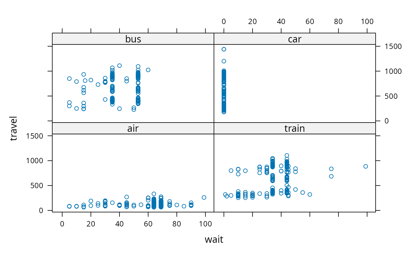
## travel vs. waiting time for different travel modes
library("lattice")
xyplot(travel ~ wait | mode, data = TravelMode)


## Greene (2003), Table 21.11, conditional logit model
library("mlogit")
TravelMode$incair <- with(TravelMode, income * (mode == "air"))
tm_cl <- mlogit(choice ~ gcost + wait + incair, data = TravelMode,
  shape = "long", alt.var = "mode", reflevel = "car")
summary(tm_cl)
#> 
#> Call:
#> mlogit(formula = choice ~ gcost + wait + incair, data = TravelMode, 
#>     reflevel = "car", shape = "long", alt.var = "mode", method = "nr")
#> 
#> Frequencies of alternatives:choice
#>     car     air   train     bus 
#> 0.28095 0.27619 0.30000 0.14286 
#> 
#> nr method
#> 5 iterations, 0h:0m:0s 
#> g'(-H)^-1g = 0.000234 
#> successive function values within tolerance limits 
#> 
#> Coefficients :
#>                    Estimate Std. Error z-value  Pr(>|z|)    
#> (Intercept):air    5.207433   0.779055  6.6843 2.320e-11 ***
#> (Intercept):train  3.869036   0.443127  8.7312 < 2.2e-16 ***
#> (Intercept):bus    3.163190   0.450266  7.0252 2.138e-12 ***
#> gcost             -0.015501   0.004408 -3.5167  0.000437 ***
#> wait              -0.096125   0.010440 -9.2075 < 2.2e-16 ***
#> incair             0.013287   0.010262  1.2947  0.195414    
#> ---
#> Signif. codes:  0 ‘***’ 0.001 ‘**’ 0.01 ‘*’ 0.05 ‘.’ 0.1 ‘ ’ 1
#> 
#> Log-Likelihood: -199.13
#> McFadden R^2:  0.29825 
#> Likelihood ratio test : chisq = 169.26 (p.value = < 2.22e-16)