Expenditure and Default Data

Cross-section data on the credit history for a sample of applicants for a type of credit card.

Usage

data("CreditCard")

Format

A data frame containing 1,319 observations on 12 variables.

card

Factor. Was the application for a credit card accepted?

reports

Number of major derogatory reports.

age

Age in years plus twelfths of a year.

income

Yearly income (in USD 10,000).

share

Ratio of monthly credit card expenditure to yearly income.

expenditure

Average monthly credit card expenditure.

owner

Factor. Does the individual own their home?

selfemp

Factor. Is the individual self-employed?

dependents

Number of dependents.

months

Months living at current address.

majorcards

Number of major credit cards held.

active

Number of active credit accounts.

Details

According to Greene (2003, p. 952) dependents equals 1 + number of dependents, our calculations suggest that it equals number of dependents.

Greene (2003) provides this data set twice in Table F21.4 and F9.1, respectively. Table F9.1 has just the observations, rounded to two digits. Here, we give the F21.4 version, see the examples for the F9.1 version. Note that age has some suspiciously low values (below one year) for some applicants. One of these differs between the F9.1 and F21.4 version.

Source

Online complements to Greene (2003). Table F21.4.

https://pages.stern.nyu.edu/~wgreene/Text/tables/tablelist5.htm

References

Greene, W.H. (2003). Econometric Analysis, 5th edition. Upper Saddle River, NJ: Prentice Hall.

See also

Greene2003

Examples

data("CreditCard")

## Greene (2003)
## extract data set F9.1
ccard <- CreditCard[1:100,]
ccard$income <- round(ccard$income, digits = 2)
ccard$expenditure <- round(ccard$expenditure, digits = 2)
ccard$age <- round(ccard$age + .01)
## suspicious:
CreditCard$age[CreditCard$age < 1]
#> [1] 0.5000000 0.1666667 0.5833333 0.7500000 0.5833333 0.5000000 0.7500000
## the first of these is also in TableF9.1 with 36 instead of 0.5:
ccard$age[79] <- 36

## Example 11.1
ccard <- ccard[order(ccard$income),]
ccard0 <- subset(ccard, expenditure > 0)
cc_ols <- lm(expenditure ~ age + owner + income + I(income^2), data = ccard0)

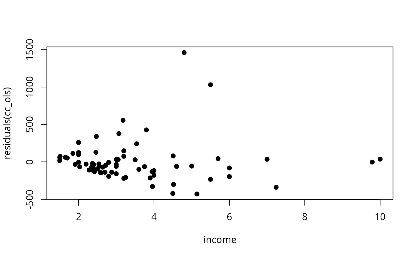
## Figure 11.1
plot(residuals(cc_ols) ~ income, data = ccard0, pch = 19)


## Table 11.1
mean(ccard$age)
#> [1] 32.08
prop.table(table(ccard$owner))
#> 
#>   no  yes 
#> 0.64 0.36 
mean(ccard$income)
#> [1] 3.3692

summary(cc_ols)
#> 
#> Call:
#> lm(formula = expenditure ~ age + owner + income + I(income^2), 
#>     data = ccard0)
#> 
#> Residuals:
#>     Min      1Q  Median      3Q     Max 
#> -429.03 -130.39  -51.14   53.96 1460.55 
#> 
#> Coefficients:
#>             Estimate Std. Error t value Pr(>|t|)   
#> (Intercept) -237.127    199.324  -1.190  0.23838   
#> age           -3.086      5.515  -0.560  0.57759   
#> owneryes      27.911     82.920   0.337  0.73747   
#> income       234.416     80.365   2.917  0.00481 **
#> I(income^2)  -15.002      7.469  -2.009  0.04861 * 
#> ---
#> Signif. codes:  0 ‘***’ 0.001 ‘**’ 0.01 ‘*’ 0.05 ‘.’ 0.1 ‘ ’ 1
#> 
#> Residual standard error: 284.7 on 67 degrees of freedom
#> Multiple R-squared:  0.2436,	Adjusted R-squared:  0.1985 
#> F-statistic: 5.396 on 4 and 67 DF,  p-value: 0.0007932
#> 
sqrt(diag(vcovHC(cc_ols, type = "HC0")))
#> (Intercept)         age    owneryes      income I(income^2) 
#>  212.953161    3.300911   92.190987   88.874353    6.945292 
sqrt(diag(vcovHC(cc_ols, type = "HC2"))) 
#> (Intercept)         age    owneryes      income I(income^2) 
#>  221.050557    3.446920   95.675689   92.092471    7.200369 
sqrt(diag(vcovHC(cc_ols, type = "HC1")))
#> (Intercept)         age    owneryes      income I(income^2) 
#>  220.756215    3.421863   95.569059   92.130897    7.199783 

bptest(cc_ols, ~ (age + income + I(income^2) + owner)^2 + I(age^2) + I(income^4), data = ccard0)
#> 
#> 	studentized Breusch-Pagan test
#> 
#> data:  cc_ols
#> BP = 14.329, df = 12, p-value = 0.2802
#> 
gqtest(cc_ols)
#> 
#> 	Goldfeld-Quandt test
#> 
#> data:  cc_ols
#> GQ = 15.004, df1 = 31, df2 = 31, p-value = 1.374e-11
#> alternative hypothesis: variance increases from segment 1 to 2
#> 
bptest(cc_ols, ~ income + I(income^2), data = ccard0, studentize = FALSE)
#> 
#> 	Breusch-Pagan test
#> 
#> data:  cc_ols
#> BP = 41.931, df = 2, p-value = 7.85e-10
#> 
bptest(cc_ols, ~ income + I(income^2), data = ccard0)
#> 
#> 	studentized Breusch-Pagan test
#> 
#> data:  cc_ols
#> BP = 6.1884, df = 2, p-value = 0.04531
#> 

## More examples can be found in:
## help("Greene2003")