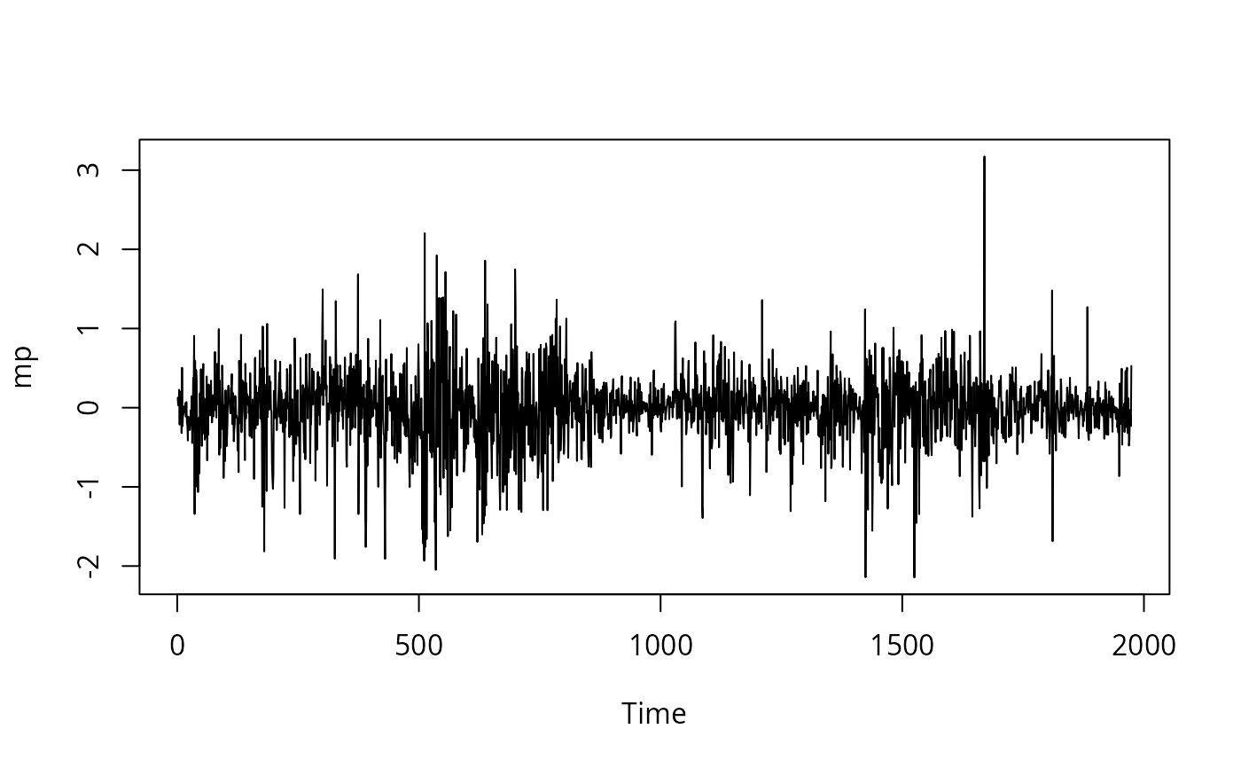
DEM/GBP Exchange Rate Returns
MarkPound.RdA daily time series of percentage returns of Deutsche mark/British pound (DEM/GBP) exchange rates from 1984-01-03 through 1991-12-31.
Usage
data("MarkPound")Format
A univariate time series of 1974 returns (exact dates unknown) for the DEM/GBP exchange rate.
Details
Greene (2003, Table F11.1) rounded the series to six digits while eight digits are given in
Bollerslev and Ghysels (1996). Here, we provide the original data. Using round
a series can be produced that is virtually identical to that of Greene (2003) (except for
eight observations where a slightly different rounding arithmetic was used).
Source
Journal of Business & Economic Statistics Data Archive.
http://www.amstat.org/publications/jbes/upload/index.cfm?fuseaction=ViewArticles&pub=JBES&issue=96-2-APR
References
Bollerslev, T., and Ghysels, E. (1996). Periodic Autoregressive Conditional Heteroskedasticity. Journal of Business & Economic Statistics, 14, 139–151.
Greene, W.H. (2003). Econometric Analysis, 5th edition. Upper Saddle River, NJ: Prentice Hall.
Examples
## data as given by Greene (2003)
data("MarkPound")
mp <- round(MarkPound, digits = 6)

## Figure 11.3 in Greene (2003)
plot(mp)


## Example 11.8 in Greene (2003), Table 11.5
library("tseries")
mp_garch <- garch(mp, grad = "numerical")
#>
#>  ***** ESTIMATION WITH NUMERICAL GRADIENT *****
#>
#>
#>      I     INITIAL X(I)        D(I)
#>
#>      1     1.990169e-01     1.000e+00
#>      2     5.000000e-02     1.000e+00
#>      3     5.000000e-02     1.000e+00
#>
#>     IT   NF      F         RELDF    PRELDF    RELDX   STPPAR   D*STEP   NPRELDF
#>      0    1 -5.449e+02
#>      1    3 -5.845e+02  6.78e-02  1.10e-01  2.5e-01  6.4e+03  1.0e-01  3.55e+02
#>      2    5 -5.913e+02  1.15e-02  3.08e-02  7.3e-02  4.6e+00  3.3e-02  4.87e+02
#>      3    6 -5.997e+02  1.40e-02  1.43e-02  7.8e-02  2.0e+00  3.3e-02  9.80e+01
#>      4    7 -6.126e+02  2.11e-02  2.71e-02  1.4e-01  2.0e+00  6.5e-02  6.24e+01
#>      5    8 -6.301e+02  2.77e-02  5.01e-02  1.8e-01  2.0e+00  1.3e-01  3.43e+01
#>      6    9 -6.537e+02  3.61e-02  4.89e-02  2.2e-01  2.0e+00  1.3e-01  1.19e+01
#>      7   11 -6.755e+02  3.24e-02  2.87e-02  1.6e-01  2.0e+00  1.3e-01  1.37e+01
#>      8   13 -6.878e+02  1.78e-02  1.71e-02  9.1e-02  2.0e+00  9.0e-02  2.84e+01
#>      9   16 -6.879e+02  2.73e-04  5.03e-04  1.4e-03  9.8e+00  1.8e-03  2.22e+01
#>     10   17 -6.881e+02  2.59e-04  2.67e-04  1.3e-03  2.1e+00  1.8e-03  1.82e+01
#>     11   18 -6.885e+02  6.02e-04  6.08e-04  2.9e-03  2.0e+00  3.6e-03  1.81e+01
#>     12   22 -6.963e+02  1.12e-02  1.21e-02  6.4e-02  2.0e+00  7.7e-02  1.73e+01
#>     13   26 -6.964e+02  1.07e-04  1.92e-04  5.9e-04  9.1e+00  8.2e-04  8.37e-01
#>     14   27 -6.965e+02  9.85e-05  1.00e-04  5.8e-04  2.4e+00  8.2e-04  6.52e-01
#>     15   28 -6.966e+02  1.80e-04  1.84e-04  1.1e-03  2.0e+00  1.6e-03  6.54e-01
#>     16   33 -7.031e+02  9.26e-03  1.18e-02  7.5e-02  1.9e+00  1.2e-01  6.40e-01
#>     17   35 -7.035e+02  5.47e-04  3.04e-03  1.3e-02  2.0e+00  1.9e-02  3.58e-01
#>     18   36 -7.039e+02  5.98e-04  4.77e-03  1.2e-02  2.0e+00  1.9e-02  1.55e-01
#>     19   37 -7.049e+02  1.45e-03  2.88e-03  1.2e-02  1.7e+00  1.9e-02  3.79e-03
#>     20   38 -7.054e+02  6.23e-04  2.27e-03  1.1e-02  1.7e+00  1.9e-02  1.82e-02
#>     21   39 -7.058e+02  5.69e-04  1.04e-03  1.1e-02  1.3e+00  1.9e-02  2.36e-03
#>     22   41 -7.064e+02  8.39e-04  9.73e-04  2.4e-02  3.0e-01  4.6e-02  1.01e-03
#>     23   42 -7.064e+02  1.88e-05  1.27e-04  4.7e-03  0.0e+00  8.2e-03  1.27e-04
#>     24   43 -7.064e+02  4.80e-05  4.67e-05  1.2e-03  0.0e+00  2.1e-03  4.67e-05
#>     25   44 -7.064e+02  4.71e-07  9.35e-07  7.7e-04  0.0e+00  1.5e-03  9.35e-07
#>     26   45 -7.064e+02  1.82e-07  2.02e-07  1.6e-04  0.0e+00  2.9e-04  2.02e-07
#>     27   46 -7.064e+02  5.22e-09  6.74e-09  4.1e-05  0.0e+00  9.0e-05  6.74e-09
#>     28   47 -7.064e+02  3.70e-10  3.72e-10  1.3e-05  0.0e+00  2.8e-05  3.72e-10
#>     29   48 -7.064e+02  1.97e-13  2.13e-13  1.6e-07  0.0e+00  3.1e-07  2.13e-13
#>
#>  ***** RELATIVE FUNCTION CONVERGENCE *****
#>
#>  FUNCTION    -7.064122e+02   RELDX        1.604e-07
#>  FUNC. EVALS      48         GRAD. EVALS     103
#>  PRELDF       2.127e-13      NPRELDF      2.127e-13
#>
#>      I      FINAL X(I)        D(I)          G(I)
#>
#>      1    1.086690e-02     1.000e+00     9.277e-04
#>      2    1.546040e-01     1.000e+00     4.473e-05
#>      3    8.044204e-01     1.000e+00     9.389e-05
#>
summary(mp_garch)
#>
#> Call:
#> garch(x = mp, grad = "numerical")
#>
#> Model:
#> GARCH(1,1)
#>
#> Residuals:
#>       Min        1Q    Median        3Q       Max
#> -6.797391 -0.537032 -0.002637  0.552328  5.248670
#>
#> Coefficient(s):
#>     Estimate  Std. Error  t value Pr(>|t|)
#> a0  0.010867    0.001297    8.376   <2e-16 ***
#> a1  0.154604    0.013882   11.137   <2e-16 ***
#> b1  0.804420    0.016046   50.133   <2e-16 ***
#> ---
#> Signif. codes:  0 ‘***’ 0.001 ‘**’ 0.01 ‘*’ 0.05 ‘.’ 0.1 ‘ ’ 1
#>
#> Diagnostic Tests:
#> 	Jarque Bera Test
#>
#> data:  Residuals
#> X-squared = 1060, df = 2, p-value < 2.2e-16
#>
#>
#> 	Box-Ljung test
#>
#> data:  Squared.Residuals
#> X-squared = 2.4776, df = 1, p-value = 0.1155
#>
logLik(mp_garch)
#> 'log Lik.' -1106.654 (df=3)
## Greene (2003) also includes a constant and uses different
## standard errors (presumably computed from Hessian), here
## OPG standard errors are used. garchFit() in "fGarch"
## implements the approach used by Greene (2003).

## compare Errata to Greene (2003)
library("dynlm")
res <- residuals(dynlm(mp ~ 1))^2
mp_ols <- dynlm(res ~ L(res, 1:10))
summary(mp_ols)
#>
#> Time series regression with "ts" data:
#> Start = 11, End = 1974
#>
#> Call:
#> dynlm(formula = res ~ L(res, 1:10))
#>
#> Residuals:
#>     Min      1Q  Median      3Q     Max
#> -1.4937 -0.1560 -0.1042 -0.0065  9.7787
#>
#> Coefficients:
#>                 Estimate Std. Error t value Pr(>|t|)
#> (Intercept)     0.095733   0.014931   6.412 1.80e-10 ***
#> L(res, 1:10)1   0.161696   0.022595   7.156 1.17e-12 ***
#> L(res, 1:10)2   0.094938   0.022882   4.149 3.48e-05 ***
#> L(res, 1:10)3   0.051267   0.022973   2.232   0.0258 *
#> L(res, 1:10)4   0.034278   0.023003   1.490   0.1363
#> L(res, 1:10)5   0.121759   0.023015   5.290 1.36e-07 ***
#> L(res, 1:10)6  -0.007805   0.023015  -0.339   0.7346
#> L(res, 1:10)7   0.003673   0.023003   0.160   0.8731
#> L(res, 1:10)8   0.029509   0.022974   1.284   0.1991
#> L(res, 1:10)9   0.025063   0.022883   1.095   0.2735
#> L(res, 1:10)10  0.054212   0.022595   2.399   0.0165 *
#> ---
#> Signif. codes:  0 ‘***’ 0.001 ‘**’ 0.01 ‘*’ 0.05 ‘.’ 0.1 ‘ ’ 1
#>
#> Residual standard error: 0.5005 on 1953 degrees of freedom
#> Multiple R-squared:  0.09795,	Adjusted R-squared:  0.09333
#> F-statistic: 21.21 on 10 and 1953 DF,  p-value: < 2.2e-16
#>
logLik(mp_ols)
#> 'log Lik.' -1421.871 (df=12)
summary(mp_ols)$r.squared * length(residuals(mp_ols))
#> [1] 192.3783
## Example 11.8 in Greene (2003), Table 11.5
library("tseries")
mp_garch <- garch(mp, grad = "numerical")
#>
#> ***** ESTIMATION WITH NUMERICAL GRADIENT *****
#>
#>
#> I INITIAL X(I) D(I)
#>
#> 1 1.990169e-01 1.000e+00
#> 2 5.000000e-02 1.000e+00
#> 3 5.000000e-02 1.000e+00
#>
#> IT NF F RELDF PRELDF RELDX STPPAR D*STEP NPRELDF
#> 0 1 -5.449e+02
#> 1 3 -5.845e+02 6.78e-02 1.10e-01 2.5e-01 6.4e+03 1.0e-01 3.55e+02
#> 2 5 -5.913e+02 1.15e-02 3.08e-02 7.3e-02 4.6e+00 3.3e-02 4.87e+02
#> 3 6 -5.997e+02 1.40e-02 1.43e-02 7.8e-02 2.0e+00 3.3e-02 9.80e+01
#> 4 7 -6.126e+02 2.11e-02 2.71e-02 1.4e-01 2.0e+00 6.5e-02 6.24e+01
#> 5 8 -6.301e+02 2.77e-02 5.01e-02 1.8e-01 2.0e+00 1.3e-01 3.43e+01
#> 6 9 -6.537e+02 3.61e-02 4.89e-02 2.2e-01 2.0e+00 1.3e-01 1.19e+01
#> 7 11 -6.755e+02 3.24e-02 2.87e-02 1.6e-01 2.0e+00 1.3e-01 1.37e+01
#> 8 13 -6.878e+02 1.78e-02 1.71e-02 9.1e-02 2.0e+00 9.0e-02 2.84e+01
#> 9 16 -6.879e+02 2.73e-04 5.03e-04 1.4e-03 9.8e+00 1.8e-03 2.22e+01
#> 10 17 -6.881e+02 2.59e-04 2.67e-04 1.3e-03 2.1e+00 1.8e-03 1.82e+01
#> 11 18 -6.885e+02 6.02e-04 6.08e-04 2.9e-03 2.0e+00 3.6e-03 1.81e+01
#> 12 22 -6.963e+02 1.12e-02 1.21e-02 6.4e-02 2.0e+00 7.7e-02 1.73e+01
#> 13 26 -6.964e+02 1.07e-04 1.92e-04 5.9e-04 9.1e+00 8.2e-04 8.37e-01
#> 14 27 -6.965e+02 9.85e-05 1.00e-04 5.8e-04 2.4e+00 8.2e-04 6.52e-01
#> 15 28 -6.966e+02 1.80e-04 1.84e-04 1.1e-03 2.0e+00 1.6e-03 6.54e-01
#> 16 33 -7.031e+02 9.26e-03 1.18e-02 7.5e-02 1.9e+00 1.2e-01 6.40e-01
#> 17 35 -7.035e+02 5.47e-04 3.04e-03 1.3e-02 2.0e+00 1.9e-02 3.58e-01
#> 18 36 -7.039e+02 5.98e-04 4.77e-03 1.2e-02 2.0e+00 1.9e-02 1.55e-01
#> 19 37 -7.049e+02 1.45e-03 2.88e-03 1.2e-02 1.7e+00 1.9e-02 3.79e-03
#> 20 38 -7.054e+02 6.23e-04 2.27e-03 1.1e-02 1.7e+00 1.9e-02 1.82e-02
#> 21 39 -7.058e+02 5.69e-04 1.04e-03 1.1e-02 1.3e+00 1.9e-02 2.36e-03
#> 22 41 -7.064e+02 8.39e-04 9.73e-04 2.4e-02 3.0e-01 4.6e-02 1.01e-03
#> 23 42 -7.064e+02 1.88e-05 1.27e-04 4.7e-03 0.0e+00 8.2e-03 1.27e-04
#> 24 43 -7.064e+02 4.80e-05 4.67e-05 1.2e-03 0.0e+00 2.1e-03 4.67e-05
#> 25 44 -7.064e+02 4.71e-07 9.35e-07 7.7e-04 0.0e+00 1.5e-03 9.35e-07
#> 26 45 -7.064e+02 1.82e-07 2.02e-07 1.6e-04 0.0e+00 2.9e-04 2.02e-07
#> 27 46 -7.064e+02 5.22e-09 6.74e-09 4.1e-05 0.0e+00 9.0e-05 6.74e-09
#> 28 47 -7.064e+02 3.70e-10 3.72e-10 1.3e-05 0.0e+00 2.8e-05 3.72e-10
#> 29 48 -7.064e+02 1.97e-13 2.13e-13 1.6e-07 0.0e+00 3.1e-07 2.13e-13
#>
#> ***** RELATIVE FUNCTION CONVERGENCE *****
#>
#> FUNCTION -7.064122e+02 RELDX 1.604e-07
#> FUNC. EVALS 48 GRAD. EVALS 103
#> PRELDF 2.127e-13 NPRELDF 2.127e-13
#>
#> I FINAL X(I) D(I) G(I)
#>
#> 1 1.086690e-02 1.000e+00 9.277e-04
#> 2 1.546040e-01 1.000e+00 4.473e-05
#> 3 8.044204e-01 1.000e+00 9.389e-05
#>
summary(mp_garch)
#>
#> Call:
#> garch(x = mp, grad = "numerical")
#>
#> Model:
#> GARCH(1,1)
#>
#> Residuals:
#> Min 1Q Median 3Q Max
#> -6.797391 -0.537032 -0.002637 0.552328 5.248670
#>
#> Coefficient(s):
#> Estimate Std. Error t value Pr(>|t|)
#> a0 0.010867 0.001297 8.376 <2e-16 ***
#> a1 0.154604 0.013882 11.137 <2e-16 ***
#> b1 0.804420 0.016046 50.133 <2e-16 ***
#> ---
#> Signif. codes: 0 ‘***’ 0.001 ‘**’ 0.01 ‘*’ 0.05 ‘.’ 0.1 ‘ ’ 1
#>
#> Diagnostic Tests:
#> Jarque Bera Test
#>
#> data: Residuals
#> X-squared = 1060, df = 2, p-value < 2.2e-16
#>
#>
#> Box-Ljung test
#>
#> data: Squared.Residuals
#> X-squared = 2.4776, df = 1, p-value = 0.1155
#>
logLik(mp_garch)
#> 'log Lik.' -1106.654 (df=3)
## Greene (2003) also includes a constant and uses different
## standard errors (presumably computed from Hessian), here
## OPG standard errors are used. garchFit() in "fGarch"
## implements the approach used by Greene (2003).
## compare Errata to Greene (2003)
library("dynlm")
res <- residuals(dynlm(mp ~ 1))^2
mp_ols <- dynlm(res ~ L(res, 1:10))
summary(mp_ols)
#>
#> Time series regression with "ts" data:
#> Start = 11, End = 1974
#>
#> Call:
#> dynlm(formula = res ~ L(res, 1:10))
#>
#> Residuals:
#> Min 1Q Median 3Q Max
#> -1.4937 -0.1560 -0.1042 -0.0065 9.7787
#>
#> Coefficients:
#> Estimate Std. Error t value Pr(>|t|)
#> (Intercept) 0.095733 0.014931 6.412 1.80e-10 ***
#> L(res, 1:10)1 0.161696 0.022595 7.156 1.17e-12 ***
#> L(res, 1:10)2 0.094938 0.022882 4.149 3.48e-05 ***
#> L(res, 1:10)3 0.051267 0.022973 2.232 0.0258 *
#> L(res, 1:10)4 0.034278 0.023003 1.490 0.1363
#> L(res, 1:10)5 0.121759 0.023015 5.290 1.36e-07 ***
#> L(res, 1:10)6 -0.007805 0.023015 -0.339 0.7346
#> L(res, 1:10)7 0.003673 0.023003 0.160 0.8731
#> L(res, 1:10)8 0.029509 0.022974 1.284 0.1991
#> L(res, 1:10)9 0.025063 0.022883 1.095 0.2735
#> L(res, 1:10)10 0.054212 0.022595 2.399 0.0165 *
#> ---
#> Signif. codes: 0 ‘***’ 0.001 ‘**’ 0.01 ‘*’ 0.05 ‘.’ 0.1 ‘ ’ 1
#>
#> Residual standard error: 0.5005 on 1953 degrees of freedom
#> Multiple R-squared: 0.09795, Adjusted R-squared: 0.09333
#> F-statistic: 21.21 on 10 and 1953 DF, p-value: < 2.2e-16
#>
logLik(mp_ols)
#> 'log Lik.' -1421.871 (df=12)
summary(mp_ols)$r.squared * length(residuals(mp_ols))
#> [1] 192.3783