US Gasoline Market Data (1960–1995, Greene)
USGasG.RdTime series data on the US gasoline market.
Usage
data("USGasG")Format
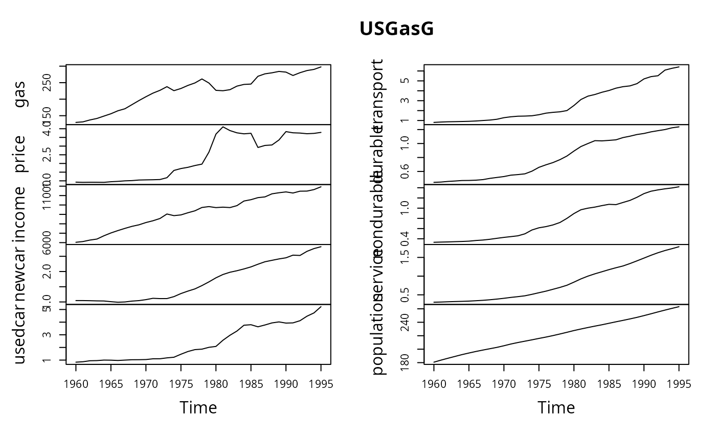
An annual multiple time series from 1960 to 1995 with 10 variables.
- gas
Total US gasoline consumption (computed as total expenditure divided by price index).
- price
Price index for gasoline.
- income
Per capita disposable income.
- newcar
Price index for new cars.
- usedcar
Price index for used cars.
- transport
Price index for public transportation.
- durable
Aggregate price index for consumer durables.
- nondurable
Aggregate price index for consumer nondurables.
- service
Aggregate price index for consumer services.
- population
US total population in millions.
Source
Online complements to Greene (2003). Table F2.2.
https://pages.stern.nyu.edu/~wgreene/Text/tables/tablelist5.htm
References
Greene, W.H. (2003). Econometric Analysis, 5th edition. Upper Saddle River, NJ: Prentice Hall.
Examples
data("USGasG", package = "AER")
plot(USGasG)
 ## Greene (2003)
## Example 2.3
fm <- lm(log(gas/population) ~ log(price) + log(income) + log(newcar) + log(usedcar),
data = as.data.frame(USGasG))
summary(fm)
#>
#> Call:
#> lm(formula = log(gas/population) ~ log(price) + log(income) +
#> log(newcar) + log(usedcar), data = as.data.frame(USGasG))
#>
#> Residuals:
#> Min 1Q Median 3Q Max
#> -0.065042 -0.018842 0.001528 0.020786 0.058084
#>
#> Coefficients:
#> Estimate Std. Error t value Pr(>|t|)
#> (Intercept) -12.34184 0.67489 -18.287 <2e-16 ***
#> log(price) -0.05910 0.03248 -1.819 0.0786 .
#> log(income) 1.37340 0.07563 18.160 <2e-16 ***
#> log(newcar) -0.12680 0.12699 -0.998 0.3258
#> log(usedcar) -0.11871 0.08134 -1.459 0.1545
#> ---
#> Signif. codes: 0 ‘***’ 0.001 ‘**’ 0.01 ‘*’ 0.05 ‘.’ 0.1 ‘ ’ 1
#>
#> Residual standard error: 0.03304 on 31 degrees of freedom
#> Multiple R-squared: 0.958, Adjusted R-squared: 0.9526
#> F-statistic: 176.7 on 4 and 31 DF, p-value: < 2.2e-16
#>
## Example 4.4
## estimates and standard errors (note different offset for intercept)
coef(fm)
#> (Intercept) log(price) log(income) log(newcar) log(usedcar)
#> -12.34184054 -0.05909513 1.37339912 -0.12679667 -0.11870847
sqrt(diag(vcov(fm)))
#> (Intercept) log(price) log(income) log(newcar) log(usedcar)
#> 0.67489471 0.03248496 0.07562767 0.12699351 0.08133710
## confidence interval
confint(fm, parm = "log(income)")
#> 2.5 % 97.5 %
#> log(income) 1.219155 1.527643
## test linear hypothesis
linearHypothesis(fm, "log(income) = 1")
#>
#> Linear hypothesis test:
#> log(income) = 1
#>
#> Model 1: restricted model
#> Model 2: log(gas/population) ~ log(price) + log(income) + log(newcar) +
#> log(usedcar)
#>
#> Res.Df RSS Df Sum of Sq F Pr(>F)
#> 1 32 0.060445
#> 2 31 0.033837 1 0.026608 24.377 2.57e-05 ***
#> ---
#> Signif. codes: 0 ‘***’ 0.001 ‘**’ 0.01 ‘*’ 0.05 ‘.’ 0.1 ‘ ’ 1
## Example 7.6
## re-used in Example 8.3
trend <- 1:nrow(USGasG)
shock <- factor(time(USGasG) > 1973, levels = c(FALSE, TRUE),
labels = c("before", "after"))
## 1960-1995
fm1 <- lm(log(gas/population) ~ log(income) + log(price) + log(newcar) +
log(usedcar) + trend, data = as.data.frame(USGasG))
summary(fm1)
#>
#> Call:
#> lm(formula = log(gas/population) ~ log(income) + log(price) +
#> log(newcar) + log(usedcar) + trend, data = as.data.frame(USGasG))
#>
#> Residuals:
#> Min 1Q Median 3Q Max
#> -0.055238 -0.017715 0.003659 0.016481 0.053522
#>
#> Coefficients:
#> Estimate Std. Error t value Pr(>|t|)
#> (Intercept) -17.385790 1.679289 -10.353 2.03e-11 ***
#> log(income) 1.954626 0.192854 10.135 3.34e-11 ***
#> log(price) -0.115530 0.033479 -3.451 0.00168 **
#> log(newcar) 0.205282 0.152019 1.350 0.18700
#> log(usedcar) -0.129274 0.071412 -1.810 0.08028 .
#> trend -0.019118 0.005957 -3.210 0.00316 **
#> ---
#> Signif. codes: 0 ‘***’ 0.001 ‘**’ 0.01 ‘*’ 0.05 ‘.’ 0.1 ‘ ’ 1
#>
#> Residual standard error: 0.02898 on 30 degrees of freedom
#> Multiple R-squared: 0.9687, Adjusted R-squared: 0.9635
#> F-statistic: 185.8 on 5 and 30 DF, p-value: < 2.2e-16
#>
## pooled
fm2 <- lm(log(gas/population) ~ shock + log(income) + log(price) + log(newcar) +
log(usedcar) + trend, data = as.data.frame(USGasG))
summary(fm2)
#>
#> Call:
#> lm(formula = log(gas/population) ~ shock + log(income) + log(price) +
#> log(newcar) + log(usedcar) + trend, data = as.data.frame(USGasG))
#>
#> Residuals:
#> Min 1Q Median 3Q Max
#> -0.045360 -0.019697 0.003931 0.015112 0.047550
#>
#> Coefficients:
#> Estimate Std. Error t value Pr(>|t|)
#> (Intercept) -16.374402 1.456263 -11.244 4.33e-12 ***
#> shockafter 0.077311 0.021872 3.535 0.00139 **
#> log(income) 1.838167 0.167258 10.990 7.43e-12 ***
#> log(price) -0.178005 0.033508 -5.312 1.06e-05 ***
#> log(newcar) 0.209842 0.129267 1.623 0.11534
#> log(usedcar) -0.128132 0.060721 -2.110 0.04359 *
#> trend -0.016862 0.005105 -3.303 0.00255 **
#> ---
#> Signif. codes: 0 ‘***’ 0.001 ‘**’ 0.01 ‘*’ 0.05 ‘.’ 0.1 ‘ ’ 1
#>
#> Residual standard error: 0.02464 on 29 degrees of freedom
#> Multiple R-squared: 0.9781, Adjusted R-squared: 0.9736
#> F-statistic: 216.3 on 6 and 29 DF, p-value: < 2.2e-16
#>
## segmented
fm3 <- lm(log(gas/population) ~ shock/(log(income) + log(price) + log(newcar) +
log(usedcar) + trend), data = as.data.frame(USGasG))
summary(fm3)
#>
#> Call:
#> lm(formula = log(gas/population) ~ shock/(log(income) + log(price) +
#> log(newcar) + log(usedcar) + trend), data = as.data.frame(USGasG))
#>
#> Residuals:
#> Min 1Q Median 3Q Max
#> -0.027349 -0.006332 0.001295 0.007159 0.022016
#>
#> Coefficients:
#> Estimate Std. Error t value Pr(>|t|)
#> (Intercept) -4.13439 5.03963 -0.820 0.420075
#> shockafter -4.74111 5.51576 -0.860 0.398538
#> shockbefore:log(income) 0.42400 0.57973 0.731 0.471633
#> shockafter:log(income) 1.01408 0.24904 4.072 0.000439 ***
#> shockbefore:log(price) 0.09455 0.24804 0.381 0.706427
#> shockafter:log(price) -0.24237 0.03490 -6.946 3.5e-07 ***
#> shockbefore:log(newcar) 0.58390 0.21670 2.695 0.012665 *
#> shockafter:log(newcar) 0.33017 0.15789 2.091 0.047277 *
#> shockbefore:log(usedcar) -0.33462 0.15215 -2.199 0.037738 *
#> shockafter:log(usedcar) -0.05537 0.04426 -1.251 0.222972
#> shockbefore:trend 0.02637 0.01762 1.497 0.147533
#> shockafter:trend -0.01262 0.00329 -3.835 0.000798 ***
#> ---
#> Signif. codes: 0 ‘***’ 0.001 ‘**’ 0.01 ‘*’ 0.05 ‘.’ 0.1 ‘ ’ 1
#>
#> Residual standard error: 0.01488 on 24 degrees of freedom
#> Multiple R-squared: 0.9934, Adjusted R-squared: 0.9904
#> F-statistic: 328.5 on 11 and 24 DF, p-value: < 2.2e-16
#>
## Chow test
anova(fm3, fm1)
#> Analysis of Variance Table
#>
#> Model 1: log(gas/population) ~ shock/(log(income) + log(price) + log(newcar) +
#> log(usedcar) + trend)
#> Model 2: log(gas/population) ~ log(income) + log(price) + log(newcar) +
#> log(usedcar) + trend
#> Res.Df RSS Df Sum of Sq F Pr(>F)
#> 1 24 0.0053144
#> 2 30 0.0251878 -6 -0.019873 14.958 4.595e-07 ***
#> ---
#> Signif. codes: 0 ‘***’ 0.001 ‘**’ 0.01 ‘*’ 0.05 ‘.’ 0.1 ‘ ’ 1
library("strucchange")
sctest(log(gas/population) ~ log(income) + log(price) + log(newcar) +
log(usedcar) + trend, data = USGasG, point = c(1973, 1), type = "Chow")
#>
#> Chow test
#>
#> data: log(gas/population) ~ log(income) + log(price) + log(newcar) + log(usedcar) + trend
#> F = 14.958, p-value = 4.595e-07
#>
## Recursive CUSUM test
rcus <- efp(log(gas/population) ~ log(income) + log(price) + log(newcar) +
log(usedcar) + trend, data = USGasG, type = "Rec-CUSUM")
plot(rcus)
## Greene (2003)
## Example 2.3
fm <- lm(log(gas/population) ~ log(price) + log(income) + log(newcar) + log(usedcar),
data = as.data.frame(USGasG))
summary(fm)
#>
#> Call:
#> lm(formula = log(gas/population) ~ log(price) + log(income) +
#> log(newcar) + log(usedcar), data = as.data.frame(USGasG))
#>
#> Residuals:
#> Min 1Q Median 3Q Max
#> -0.065042 -0.018842 0.001528 0.020786 0.058084
#>
#> Coefficients:
#> Estimate Std. Error t value Pr(>|t|)
#> (Intercept) -12.34184 0.67489 -18.287 <2e-16 ***
#> log(price) -0.05910 0.03248 -1.819 0.0786 .
#> log(income) 1.37340 0.07563 18.160 <2e-16 ***
#> log(newcar) -0.12680 0.12699 -0.998 0.3258
#> log(usedcar) -0.11871 0.08134 -1.459 0.1545
#> ---
#> Signif. codes: 0 ‘***’ 0.001 ‘**’ 0.01 ‘*’ 0.05 ‘.’ 0.1 ‘ ’ 1
#>
#> Residual standard error: 0.03304 on 31 degrees of freedom
#> Multiple R-squared: 0.958, Adjusted R-squared: 0.9526
#> F-statistic: 176.7 on 4 and 31 DF, p-value: < 2.2e-16
#>
## Example 4.4
## estimates and standard errors (note different offset for intercept)
coef(fm)
#> (Intercept) log(price) log(income) log(newcar) log(usedcar)
#> -12.34184054 -0.05909513 1.37339912 -0.12679667 -0.11870847
sqrt(diag(vcov(fm)))
#> (Intercept) log(price) log(income) log(newcar) log(usedcar)
#> 0.67489471 0.03248496 0.07562767 0.12699351 0.08133710
## confidence interval
confint(fm, parm = "log(income)")
#> 2.5 % 97.5 %
#> log(income) 1.219155 1.527643
## test linear hypothesis
linearHypothesis(fm, "log(income) = 1")
#>
#> Linear hypothesis test:
#> log(income) = 1
#>
#> Model 1: restricted model
#> Model 2: log(gas/population) ~ log(price) + log(income) + log(newcar) +
#> log(usedcar)
#>
#> Res.Df RSS Df Sum of Sq F Pr(>F)
#> 1 32 0.060445
#> 2 31 0.033837 1 0.026608 24.377 2.57e-05 ***
#> ---
#> Signif. codes: 0 ‘***’ 0.001 ‘**’ 0.01 ‘*’ 0.05 ‘.’ 0.1 ‘ ’ 1
## Example 7.6
## re-used in Example 8.3
trend <- 1:nrow(USGasG)
shock <- factor(time(USGasG) > 1973, levels = c(FALSE, TRUE),
labels = c("before", "after"))
## 1960-1995
fm1 <- lm(log(gas/population) ~ log(income) + log(price) + log(newcar) +
log(usedcar) + trend, data = as.data.frame(USGasG))
summary(fm1)
#>
#> Call:
#> lm(formula = log(gas/population) ~ log(income) + log(price) +
#> log(newcar) + log(usedcar) + trend, data = as.data.frame(USGasG))
#>
#> Residuals:
#> Min 1Q Median 3Q Max
#> -0.055238 -0.017715 0.003659 0.016481 0.053522
#>
#> Coefficients:
#> Estimate Std. Error t value Pr(>|t|)
#> (Intercept) -17.385790 1.679289 -10.353 2.03e-11 ***
#> log(income) 1.954626 0.192854 10.135 3.34e-11 ***
#> log(price) -0.115530 0.033479 -3.451 0.00168 **
#> log(newcar) 0.205282 0.152019 1.350 0.18700
#> log(usedcar) -0.129274 0.071412 -1.810 0.08028 .
#> trend -0.019118 0.005957 -3.210 0.00316 **
#> ---
#> Signif. codes: 0 ‘***’ 0.001 ‘**’ 0.01 ‘*’ 0.05 ‘.’ 0.1 ‘ ’ 1
#>
#> Residual standard error: 0.02898 on 30 degrees of freedom
#> Multiple R-squared: 0.9687, Adjusted R-squared: 0.9635
#> F-statistic: 185.8 on 5 and 30 DF, p-value: < 2.2e-16
#>
## pooled
fm2 <- lm(log(gas/population) ~ shock + log(income) + log(price) + log(newcar) +
log(usedcar) + trend, data = as.data.frame(USGasG))
summary(fm2)
#>
#> Call:
#> lm(formula = log(gas/population) ~ shock + log(income) + log(price) +
#> log(newcar) + log(usedcar) + trend, data = as.data.frame(USGasG))
#>
#> Residuals:
#> Min 1Q Median 3Q Max
#> -0.045360 -0.019697 0.003931 0.015112 0.047550
#>
#> Coefficients:
#> Estimate Std. Error t value Pr(>|t|)
#> (Intercept) -16.374402 1.456263 -11.244 4.33e-12 ***
#> shockafter 0.077311 0.021872 3.535 0.00139 **
#> log(income) 1.838167 0.167258 10.990 7.43e-12 ***
#> log(price) -0.178005 0.033508 -5.312 1.06e-05 ***
#> log(newcar) 0.209842 0.129267 1.623 0.11534
#> log(usedcar) -0.128132 0.060721 -2.110 0.04359 *
#> trend -0.016862 0.005105 -3.303 0.00255 **
#> ---
#> Signif. codes: 0 ‘***’ 0.001 ‘**’ 0.01 ‘*’ 0.05 ‘.’ 0.1 ‘ ’ 1
#>
#> Residual standard error: 0.02464 on 29 degrees of freedom
#> Multiple R-squared: 0.9781, Adjusted R-squared: 0.9736
#> F-statistic: 216.3 on 6 and 29 DF, p-value: < 2.2e-16
#>
## segmented
fm3 <- lm(log(gas/population) ~ shock/(log(income) + log(price) + log(newcar) +
log(usedcar) + trend), data = as.data.frame(USGasG))
summary(fm3)
#>
#> Call:
#> lm(formula = log(gas/population) ~ shock/(log(income) + log(price) +
#> log(newcar) + log(usedcar) + trend), data = as.data.frame(USGasG))
#>
#> Residuals:
#> Min 1Q Median 3Q Max
#> -0.027349 -0.006332 0.001295 0.007159 0.022016
#>
#> Coefficients:
#> Estimate Std. Error t value Pr(>|t|)
#> (Intercept) -4.13439 5.03963 -0.820 0.420075
#> shockafter -4.74111 5.51576 -0.860 0.398538
#> shockbefore:log(income) 0.42400 0.57973 0.731 0.471633
#> shockafter:log(income) 1.01408 0.24904 4.072 0.000439 ***
#> shockbefore:log(price) 0.09455 0.24804 0.381 0.706427
#> shockafter:log(price) -0.24237 0.03490 -6.946 3.5e-07 ***
#> shockbefore:log(newcar) 0.58390 0.21670 2.695 0.012665 *
#> shockafter:log(newcar) 0.33017 0.15789 2.091 0.047277 *
#> shockbefore:log(usedcar) -0.33462 0.15215 -2.199 0.037738 *
#> shockafter:log(usedcar) -0.05537 0.04426 -1.251 0.222972
#> shockbefore:trend 0.02637 0.01762 1.497 0.147533
#> shockafter:trend -0.01262 0.00329 -3.835 0.000798 ***
#> ---
#> Signif. codes: 0 ‘***’ 0.001 ‘**’ 0.01 ‘*’ 0.05 ‘.’ 0.1 ‘ ’ 1
#>
#> Residual standard error: 0.01488 on 24 degrees of freedom
#> Multiple R-squared: 0.9934, Adjusted R-squared: 0.9904
#> F-statistic: 328.5 on 11 and 24 DF, p-value: < 2.2e-16
#>
## Chow test
anova(fm3, fm1)
#> Analysis of Variance Table
#>
#> Model 1: log(gas/population) ~ shock/(log(income) + log(price) + log(newcar) +
#> log(usedcar) + trend)
#> Model 2: log(gas/population) ~ log(income) + log(price) + log(newcar) +
#> log(usedcar) + trend
#> Res.Df RSS Df Sum of Sq F Pr(>F)
#> 1 24 0.0053144
#> 2 30 0.0251878 -6 -0.019873 14.958 4.595e-07 ***
#> ---
#> Signif. codes: 0 ‘***’ 0.001 ‘**’ 0.01 ‘*’ 0.05 ‘.’ 0.1 ‘ ’ 1
library("strucchange")
sctest(log(gas/population) ~ log(income) + log(price) + log(newcar) +
log(usedcar) + trend, data = USGasG, point = c(1973, 1), type = "Chow")
#>
#> Chow test
#>
#> data: log(gas/population) ~ log(income) + log(price) + log(newcar) + log(usedcar) + trend
#> F = 14.958, p-value = 4.595e-07
#>
## Recursive CUSUM test
rcus <- efp(log(gas/population) ~ log(income) + log(price) + log(newcar) +
log(usedcar) + trend, data = USGasG, type = "Rec-CUSUM")
plot(rcus)
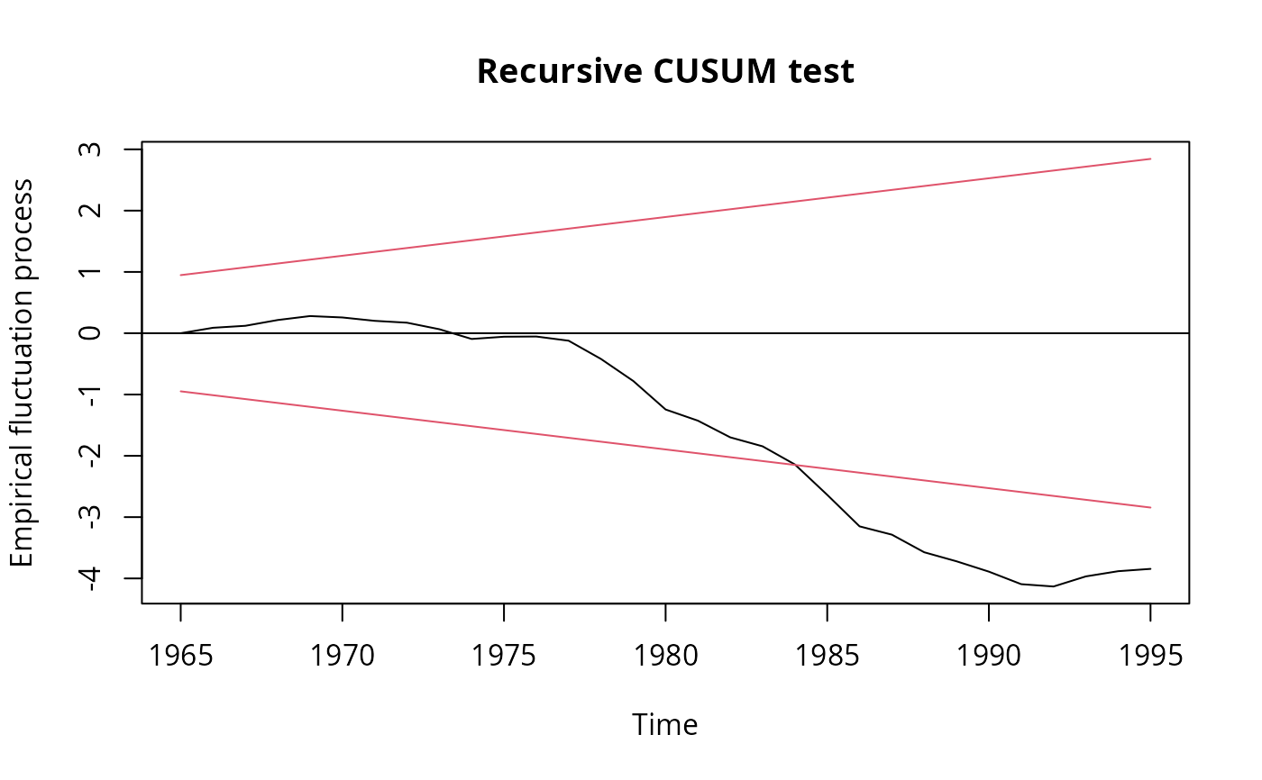 sctest(rcus)
#>
#> Recursive CUSUM test
#>
#> data: rcus
#> S = 1.4977, p-value = 0.0002437
#>
## Note: Greene's remark that the break is in 1984 (where the process crosses its
## boundary) is wrong. The break appears to be no later than 1976.
## More examples can be found in:
## help("Greene2003")
sctest(rcus)
#>
#> Recursive CUSUM test
#>
#> data: rcus
#> S = 1.4977, p-value = 0.0002437
#>
## Note: Greene's remark that the break is in 1984 (where the process crosses its
## boundary) is wrong. The break appears to be no later than 1976.
## More examples can be found in:
## help("Greene2003")