SIC33 Production Data
SIC33.RdStatewide production data for primary metals industry (SIC 33).
Usage
data("SIC33")Format
A data frame containing 27 observations on 3 variables.
- output
Value added.
- labor
Labor input.
- capital
Capital stock.
Source
Online complements to Greene (2003). Table F6.1.
https://pages.stern.nyu.edu/~wgreene/Text/tables/tablelist5.htm
References
Greene, W.H. (2003). Econometric Analysis, 5th edition. Upper Saddle River, NJ: Prentice Hall.
Examples
#> Loading required namespace: scatterplot3d
data("SIC33", package = "AER")
## Example 6.2 in Greene (2003)
## Translog model
fm_tl <- lm(output ~ labor + capital + I(0.5 * labor^2) + I(0.5 * capital^2) + I(labor * capital),
data = log(SIC33))
## Cobb-Douglas model
fm_cb <- lm(output ~ labor + capital, data = log(SIC33))
## Table 6.2 in Greene (2003)
deviance(fm_tl)
#> [1] 0.6799272
deviance(fm_cb)
#> [1] 0.8516337
summary(fm_tl)
#>
#> Call:
#> lm(formula = output ~ labor + capital + I(0.5 * labor^2) + I(0.5 *
#> capital^2) + I(labor * capital), data = log(SIC33))
#>
#> Residuals:
#> Min 1Q Median 3Q Max
#> -0.33990 -0.10106 -0.01238 0.04605 0.39281
#>
#> Coefficients:
#> Estimate Std. Error t value Pr(>|t|)
#> (Intercept) 0.94420 2.91075 0.324 0.7489
#> labor 3.61364 1.54807 2.334 0.0296 *
#> capital -1.89311 1.01626 -1.863 0.0765 .
#> I(0.5 * labor^2) -0.96405 0.70738 -1.363 0.1874
#> I(0.5 * capital^2) 0.08529 0.29261 0.291 0.7735
#> I(labor * capital) 0.31239 0.43893 0.712 0.4845
#> ---
#> Signif. codes: 0 ‘***’ 0.001 ‘**’ 0.01 ‘*’ 0.05 ‘.’ 0.1 ‘ ’ 1
#>
#> Residual standard error: 0.1799 on 21 degrees of freedom
#> Multiple R-squared: 0.9549, Adjusted R-squared: 0.9441
#> F-statistic: 88.85 on 5 and 21 DF, p-value: 2.121e-13
#>
summary(fm_cb)
#>
#> Call:
#> lm(formula = output ~ labor + capital, data = log(SIC33))
#>
#> Residuals:
#> Min 1Q Median 3Q Max
#> -0.30385 -0.10119 -0.01819 0.05582 0.50559
#>
#> Coefficients:
#> Estimate Std. Error t value Pr(>|t|)
#> (Intercept) 1.17064 0.32678 3.582 0.00150 **
#> labor 0.60300 0.12595 4.787 7.13e-05 ***
#> capital 0.37571 0.08535 4.402 0.00019 ***
#> ---
#> Signif. codes: 0 ‘***’ 0.001 ‘**’ 0.01 ‘*’ 0.05 ‘.’ 0.1 ‘ ’ 1
#>
#> Residual standard error: 0.1884 on 24 degrees of freedom
#> Multiple R-squared: 0.9435, Adjusted R-squared: 0.9388
#> F-statistic: 200.2 on 2 and 24 DF, p-value: 1.067e-15
#>
vcov(fm_tl)
#> (Intercept) labor capital I(0.5 * labor^2)
#> (Intercept) 8.47248687 -2.38790338 -0.33129294 -0.08760011
#> labor -2.38790338 2.39652901 -1.23101576 -0.66580411
#> capital -0.33129294 -1.23101576 1.03278652 0.52305244
#> I(0.5 * labor^2) -0.08760011 -0.66580411 0.52305244 0.50039330
#> I(0.5 * capital^2) -0.23317345 0.03476689 0.02636926 0.14674300
#> I(labor * capital) 0.36354446 0.18311307 -0.22554189 -0.28803386
#> I(0.5 * capital^2) I(labor * capital)
#> (Intercept) -0.23317345 0.3635445
#> labor 0.03476689 0.1831131
#> capital 0.02636926 -0.2255419
#> I(0.5 * labor^2) 0.14674300 -0.2880339
#> I(0.5 * capital^2) 0.08562001 -0.1160405
#> I(labor * capital) -0.11604045 0.1926571
vcov(fm_cb)
#> (Intercept) labor capital
#> (Intercept) 0.10678650 -0.019835398 0.001188850
#> labor -0.01983540 0.015864400 -0.009616201
#> capital 0.00118885 -0.009616201 0.007283931
## Cobb-Douglas vs. Translog model
anova(fm_cb, fm_tl)
#> Analysis of Variance Table
#>
#> Model 1: output ~ labor + capital
#> Model 2: output ~ labor + capital + I(0.5 * labor^2) + I(0.5 * capital^2) +
#> I(labor * capital)
#> Res.Df RSS Df Sum of Sq F Pr(>F)
#> 1 24 0.85163
#> 2 21 0.67993 3 0.17171 1.7678 0.1841
## hypothesis of constant returns
linearHypothesis(fm_cb, "labor + capital = 1")
#>
#> Linear hypothesis test:
#> labor + capital = 1
#>
#> Model 1: restricted model
#> Model 2: output ~ labor + capital
#>
#> Res.Df RSS Df Sum of Sq F Pr(>F)
#> 1 25 0.85574
#> 2 24 0.85163 1 0.0041075 0.1158 0.7366
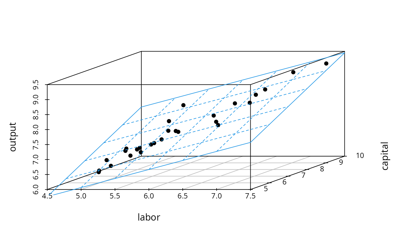
## 3D Visualization
library("scatterplot3d")
s3d <- scatterplot3d(log(SIC33)[,c(2, 3, 1)], pch = 16)
s3d$plane3d(fm_cb, lty.box = "solid", col = 4)
 ## Interactive 3D Visualization
# \donttest{
if(require("rgl")) {
x <- log(SIC33)[,2]
y <- log(SIC33)[,3]
z <- log(SIC33)[,1]
plot3d(x, y, z, type = "s", col = "gray", radius = 0.1)
x <- seq(4.5, 7.5, by = 0.5)
y <- seq(5.5, 10, by = 0.5)
z <- outer(x, y, function(x, y) predict(fm_cb, data.frame(labor = x, capital = y)))
surface3d(x, y, z, color = "blue", alpha = 0.5, shininess = 128)
}
#> Loading required package: rgl
#> Warning: RGL: unable to open X11 display
#> Warning: 'rgl.init' failed, will use the null device.
#> See '?rgl.useNULL' for ways to avoid this warning.
## Interactive 3D Visualization
# \donttest{
if(require("rgl")) {
x <- log(SIC33)[,2]
y <- log(SIC33)[,3]
z <- log(SIC33)[,1]
plot3d(x, y, z, type = "s", col = "gray", radius = 0.1)
x <- seq(4.5, 7.5, by = 0.5)
y <- seq(5.5, 10, by = 0.5)
z <- outer(x, y, function(x, y) predict(fm_cb, data.frame(labor = x, capital = y)))
surface3d(x, y, z, color = "blue", alpha = 0.5, shininess = 128)
}
#> Loading required package: rgl
#> Warning: RGL: unable to open X11 display
#> Warning: 'rgl.init' failed, will use the null device.
#> See '?rgl.useNULL' for ways to avoid this warning.
3D plot
# }