US Consumption Data (1970–1979)
USConsump1979.RdTime series data on US income and consumption expenditure, 1970–1979.
Usage
data("USConsump1979")Format
An annual multiple time series from 1970 to 1979 with 2 variables.
- income
Disposable income.
- expenditure
Consumption expenditure.
Source
Online complements to Greene (2003). Table F1.1.
https://pages.stern.nyu.edu/~wgreene/Text/tables/tablelist5.htm
References
Greene, W.H. (2003). Econometric Analysis, 5th edition. Upper Saddle River, NJ: Prentice Hall.
Examples
data("USConsump1979")
plot(USConsump1979)
 ## Example 1.1 in Greene (2003)
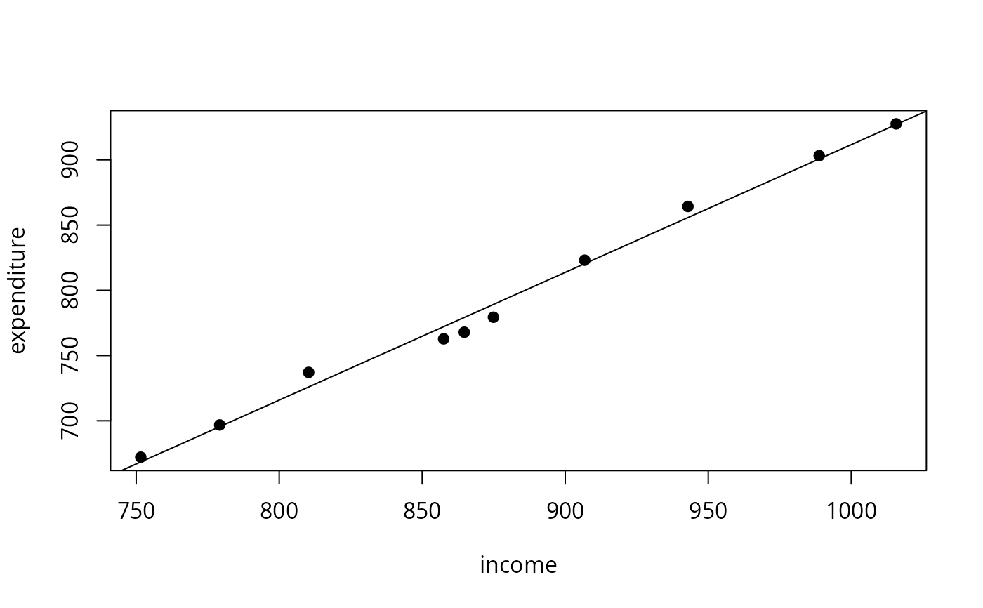
plot(expenditure ~ income, data = as.data.frame(USConsump1979), pch = 19)
fm <- lm(expenditure ~ income, data = as.data.frame(USConsump1979))
summary(fm)
#>
#> Call:
#> lm(formula = expenditure ~ income, data = as.data.frame(USConsump1979))
#>
#> Residuals:
#> Min 1Q Median 3Q Max
#> -11.291 -6.871 1.909 3.418 11.181
#>
#> Coefficients:
#> Estimate Std. Error t value Pr(>|t|)
#> (Intercept) -67.58065 27.91071 -2.421 0.0418 *
#> income 0.97927 0.03161 30.983 1.28e-09 ***
#> ---
#> Signif. codes: 0 ‘***’ 0.001 ‘**’ 0.01 ‘*’ 0.05 ‘.’ 0.1 ‘ ’ 1
#>
#> Residual standard error: 8.193 on 8 degrees of freedom
#> Multiple R-squared: 0.9917, Adjusted R-squared: 0.9907
#> F-statistic: 959.9 on 1 and 8 DF, p-value: 1.28e-09
#>
abline(fm)
## Example 1.1 in Greene (2003)
plot(expenditure ~ income, data = as.data.frame(USConsump1979), pch = 19)
fm <- lm(expenditure ~ income, data = as.data.frame(USConsump1979))
summary(fm)
#>
#> Call:
#> lm(formula = expenditure ~ income, data = as.data.frame(USConsump1979))
#>
#> Residuals:
#> Min 1Q Median 3Q Max
#> -11.291 -6.871 1.909 3.418 11.181
#>
#> Coefficients:
#> Estimate Std. Error t value Pr(>|t|)
#> (Intercept) -67.58065 27.91071 -2.421 0.0418 *
#> income 0.97927 0.03161 30.983 1.28e-09 ***
#> ---
#> Signif. codes: 0 ‘***’ 0.001 ‘**’ 0.01 ‘*’ 0.05 ‘.’ 0.1 ‘ ’ 1
#>
#> Residual standard error: 8.193 on 8 degrees of freedom
#> Multiple R-squared: 0.9917, Adjusted R-squared: 0.9907
#> F-statistic: 959.9 on 1 and 8 DF, p-value: 1.28e-09
#>
abline(fm)