US Consumption Data (1940–1950)
USConsump1950.RdTime series data on US income and consumption expenditure, 1940–1950.
Usage
data("USConsump1950")Format
An annual multiple time series from 1940 to 1950 with 3 variables.
- income
Disposable income.
- expenditure
Consumption expenditure.
- war
Indicator variable: Was the year a year of war?
Source
Online complements to Greene (2003). Table F2.1.
https://pages.stern.nyu.edu/~wgreene/Text/tables/tablelist5.htm
References
Greene, W.H. (2003). Econometric Analysis, 5th edition. Upper Saddle River, NJ: Prentice Hall.
Examples
## Greene (2003)
## data
data("USConsump1950")
usc <- as.data.frame(USConsump1950)
usc$war <- factor(usc$war, labels = c("no", "yes"))
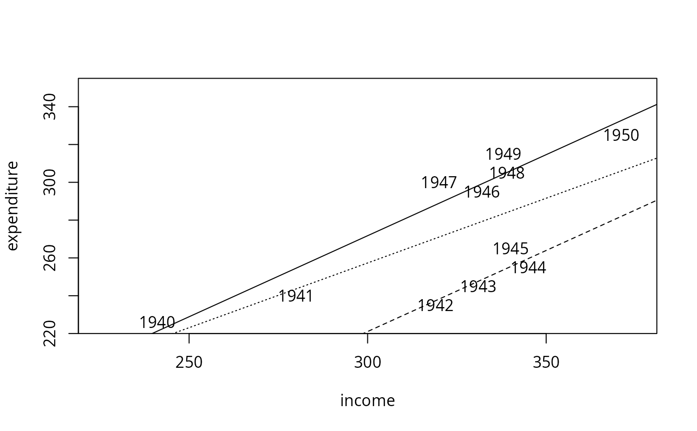
## Example 2.1
plot(expenditure ~ income, data = usc, type = "n", xlim = c(225, 375), ylim = c(225, 350))
with(usc, text(income, expenditure, time(USConsump1950)))
## single model
fm <- lm(expenditure ~ income, data = usc)
summary(fm)
#>
#> Call:
#> lm(formula = expenditure ~ income, data = usc)
#>
#> Residuals:
#> Min 1Q Median 3Q Max
#> -35.347 -26.440 9.068 20.000 31.642
#>
#> Coefficients:
#> Estimate Std. Error t value Pr(>|t|)
#> (Intercept) 51.8951 80.8440 0.642 0.5369
#> income 0.6848 0.2488 2.753 0.0224 *
#> ---
#> Signif. codes: 0 ‘***’ 0.001 ‘**’ 0.01 ‘*’ 0.05 ‘.’ 0.1 ‘ ’ 1
#>
#> Residual standard error: 27.59 on 9 degrees of freedom
#> Multiple R-squared: 0.4571, Adjusted R-squared: 0.3968
#> F-statistic: 7.579 on 1 and 9 DF, p-value: 0.02237
#>
## different intercepts for war yes/no
fm2 <- lm(expenditure ~ income + war, data = usc)
summary(fm2)
#>
#> Call:
#> lm(formula = expenditure ~ income + war, data = usc)
#>
#> Residuals:
#> Min 1Q Median 3Q Max
#> -14.598 -4.418 -2.352 7.242 11.101
#>
#> Coefficients:
#> Estimate Std. Error t value Pr(>|t|)
#> (Intercept) 14.49540 27.29948 0.531 0.61
#> income 0.85751 0.08534 10.048 8.19e-06 ***
#> waryes -50.68974 5.93237 -8.545 2.71e-05 ***
#> ---
#> Signif. codes: 0 ‘***’ 0.001 ‘**’ 0.01 ‘*’ 0.05 ‘.’ 0.1 ‘ ’ 1
#>
#> Residual standard error: 9.195 on 8 degrees of freedom
#> Multiple R-squared: 0.9464, Adjusted R-squared: 0.933
#> F-statistic: 70.61 on 2 and 8 DF, p-value: 8.26e-06
#>
## compare
anova(fm, fm2)
#> Analysis of Variance Table
#>
#> Model 1: expenditure ~ income
#> Model 2: expenditure ~ income + war
#> Res.Df RSS Df Sum of Sq F Pr(>F)
#> 1 9 6850.0
#> 2 8 676.5 1 6173.5 73.01 2.71e-05 ***
#> ---
#> Signif. codes: 0 ‘***’ 0.001 ‘**’ 0.01 ‘*’ 0.05 ‘.’ 0.1 ‘ ’ 1
## visualize
abline(fm, lty = 3)
abline(coef(fm2)[1:2])
abline(sum(coef(fm2)[c(1, 3)]), coef(fm2)[2], lty = 2)
 ## Example 3.2
summary(fm)$r.squared
#> [1] 0.4571345
summary(lm(expenditure ~ income, data = usc, subset = war == "no"))$r.squared
#> [1] 0.9369742
summary(fm2)$r.squared
#> [1] 0.9463904
## Example 3.2
summary(fm)$r.squared
#> [1] 0.4571345
summary(lm(expenditure ~ income, data = usc, subset = war == "no"))$r.squared
#> [1] 0.9369742
summary(fm2)$r.squared
#> [1] 0.9463904