Klein Model I
KleinI.RdKlein's Model I for the US economy.
Usage
data("KleinI")Format
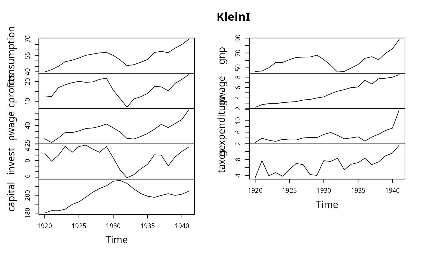
An annual multiple time series from 1920 to 1941 with 9 variables.
- consumption
Consumption.
- cprofits
Corporate profits.
- pwage
Private wage bill.
- invest
Investment.
- capital
Previous year's capital stock.
- gnp
Gross national product.
- gwage
Government wage bill.
- gexpenditure
Government spending.
- taxes
Taxes.
Source
Online complements to Greene (2003). Table F15.1.
https://pages.stern.nyu.edu/~wgreene/Text/tables/tablelist5.htm
References
Greene, W.H. (2003). Econometric Analysis, 5th edition. Upper Saddle River, NJ: Prentice Hall.
Klein, L. (1950). Economic Fluctuations in the United States, 1921–1941. New York: John Wiley.
Maddala, G.S. (1977). Econometrics. New York: McGraw-Hill.
Examples
data("KleinI", package = "AER")
plot(KleinI)


## Greene (2003), Tab. 15.3, OLS
library("dynlm")
fm_cons <- dynlm(consumption ~ cprofits + L(cprofits) + I(pwage + gwage), data = KleinI)
fm_inv <- dynlm(invest ~ cprofits + L(cprofits) + capital, data = KleinI)
fm_pwage <- dynlm(pwage ~ gnp + L(gnp) + I(time(gnp) - 1931), data = KleinI)
summary(fm_cons)
#>
#> Time series regression with "ts" data:
#> Start = 1921, End = 1941
#>
#> Call:
#> dynlm(formula = consumption ~ cprofits + L(cprofits) + I(pwage +
#>     gwage), data = KleinI)
#>
#> Residuals:
#>      Min       1Q   Median       3Q      Max
#> -2.17345 -0.43597 -0.03466  0.78508  1.61650
#>
#> Coefficients:
#>                  Estimate Std. Error t value Pr(>|t|)
#> (Intercept)      16.23660    1.30270  12.464 5.62e-10 ***
#> cprofits          0.19293    0.09121   2.115   0.0495 *
#> L(cprofits)       0.08988    0.09065   0.992   0.3353
#> I(pwage + gwage)  0.79622    0.03994  19.933 3.16e-13 ***
#> ---
#> Signif. codes:  0 ‘***’ 0.001 ‘**’ 0.01 ‘*’ 0.05 ‘.’ 0.1 ‘ ’ 1
#>
#> Residual standard error: 1.026 on 17 degrees of freedom
#> Multiple R-squared:  0.981,	Adjusted R-squared:  0.9777
#> F-statistic: 292.7 on 3 and 17 DF,  p-value: 7.938e-15
#>
summary(fm_inv)
#>
#> Time series regression with "ts" data:
#> Start = 1921, End = 1941
#>
#> Call:
#> dynlm(formula = invest ~ cprofits + L(cprofits) + capital, data = KleinI)
#>
#> Residuals:
#>      Min       1Q   Median       3Q      Max
#> -2.56562 -0.63169  0.03687  0.41542  1.49226
#>
#> Coefficients:
#>             Estimate Std. Error t value Pr(>|t|)
#> (Intercept) 10.12579    5.46555   1.853 0.081374 .
#> cprofits     0.47964    0.09711   4.939 0.000125 ***
#> L(cprofits)  0.33304    0.10086   3.302 0.004212 **
#> capital     -0.11179    0.02673  -4.183 0.000624 ***
#> ---
#> Signif. codes:  0 ‘***’ 0.001 ‘**’ 0.01 ‘*’ 0.05 ‘.’ 0.1 ‘ ’ 1
#>
#> Residual standard error: 1.009 on 17 degrees of freedom
#> Multiple R-squared:  0.9313,	Adjusted R-squared:  0.9192
#> F-statistic: 76.88 on 3 and 17 DF,  p-value: 4.299e-10
#>
summary(fm_pwage)
#>
#> Time series regression with "ts" data:
#> Start = 1921, End = 1941
#>
#> Call:
#> dynlm(formula = pwage ~ gnp + L(gnp) + I(time(gnp) - 1931), data = KleinI)
#>
#> Residuals:
#>      Min       1Q   Median       3Q      Max
#> -1.29418 -0.46875  0.01376  0.45027  1.19569
#>
#> Coefficients:
#>                     Estimate Std. Error t value Pr(>|t|)
#> (Intercept)          1.49704    1.27003   1.179 0.254736
#> gnp                  0.43948    0.03241  13.561 1.52e-10 ***
#> L(gnp)               0.14609    0.03742   3.904 0.001142 **
#> I(time(gnp) - 1931)  0.13025    0.03191   4.082 0.000777 ***
#> ---
#> Signif. codes:  0 ‘***’ 0.001 ‘**’ 0.01 ‘*’ 0.05 ‘.’ 0.1 ‘ ’ 1
#>
#> Residual standard error: 0.7671 on 17 degrees of freedom
#> Multiple R-squared:  0.9874,	Adjusted R-squared:  0.9852
#> F-statistic: 444.6 on 3 and 17 DF,  p-value: 2.411e-16
#>

## More examples can be found in:
## help("Greene2003")
## Greene (2003), Tab. 15.3, OLS
library("dynlm")
fm_cons <- dynlm(consumption ~ cprofits + L(cprofits) + I(pwage + gwage), data = KleinI)
fm_inv <- dynlm(invest ~ cprofits + L(cprofits) + capital, data = KleinI)
fm_pwage <- dynlm(pwage ~ gnp + L(gnp) + I(time(gnp) - 1931), data = KleinI)
summary(fm_cons)
#>
#> Time series regression with "ts" data:
#> Start = 1921, End = 1941
#>
#> Call:
#> dynlm(formula = consumption ~ cprofits + L(cprofits) + I(pwage +
#> gwage), data = KleinI)
#>
#> Residuals:
#> Min 1Q Median 3Q Max
#> -2.17345 -0.43597 -0.03466 0.78508 1.61650
#>
#> Coefficients:
#> Estimate Std. Error t value Pr(>|t|)
#> (Intercept) 16.23660 1.30270 12.464 5.62e-10 ***
#> cprofits 0.19293 0.09121 2.115 0.0495 *
#> L(cprofits) 0.08988 0.09065 0.992 0.3353
#> I(pwage + gwage) 0.79622 0.03994 19.933 3.16e-13 ***
#> ---
#> Signif. codes: 0 ‘***’ 0.001 ‘**’ 0.01 ‘*’ 0.05 ‘.’ 0.1 ‘ ’ 1
#>
#> Residual standard error: 1.026 on 17 degrees of freedom
#> Multiple R-squared: 0.981, Adjusted R-squared: 0.9777
#> F-statistic: 292.7 on 3 and 17 DF, p-value: 7.938e-15
#>
summary(fm_inv)
#>
#> Time series regression with "ts" data:
#> Start = 1921, End = 1941
#>
#> Call:
#> dynlm(formula = invest ~ cprofits + L(cprofits) + capital, data = KleinI)
#>
#> Residuals:
#> Min 1Q Median 3Q Max
#> -2.56562 -0.63169 0.03687 0.41542 1.49226
#>
#> Coefficients:
#> Estimate Std. Error t value Pr(>|t|)
#> (Intercept) 10.12579 5.46555 1.853 0.081374 .
#> cprofits 0.47964 0.09711 4.939 0.000125 ***
#> L(cprofits) 0.33304 0.10086 3.302 0.004212 **
#> capital -0.11179 0.02673 -4.183 0.000624 ***
#> ---
#> Signif. codes: 0 ‘***’ 0.001 ‘**’ 0.01 ‘*’ 0.05 ‘.’ 0.1 ‘ ’ 1
#>
#> Residual standard error: 1.009 on 17 degrees of freedom
#> Multiple R-squared: 0.9313, Adjusted R-squared: 0.9192
#> F-statistic: 76.88 on 3 and 17 DF, p-value: 4.299e-10
#>
summary(fm_pwage)
#>
#> Time series regression with "ts" data:
#> Start = 1921, End = 1941
#>
#> Call:
#> dynlm(formula = pwage ~ gnp + L(gnp) + I(time(gnp) - 1931), data = KleinI)
#>
#> Residuals:
#> Min 1Q Median 3Q Max
#> -1.29418 -0.46875 0.01376 0.45027 1.19569
#>
#> Coefficients:
#> Estimate Std. Error t value Pr(>|t|)
#> (Intercept) 1.49704 1.27003 1.179 0.254736
#> gnp 0.43948 0.03241 13.561 1.52e-10 ***
#> L(gnp) 0.14609 0.03742 3.904 0.001142 **
#> I(time(gnp) - 1931) 0.13025 0.03191 4.082 0.000777 ***
#> ---
#> Signif. codes: 0 ‘***’ 0.001 ‘**’ 0.01 ‘*’ 0.05 ‘.’ 0.1 ‘ ’ 1
#>
#> Residual standard error: 0.7671 on 17 degrees of freedom
#> Multiple R-squared: 0.9874, Adjusted R-squared: 0.9852
#> F-statistic: 444.6 on 3 and 17 DF, p-value: 2.411e-16
#>
## More examples can be found in:
## help("Greene2003")