Added-Variable Plots

These functions construct added-variable, also called partial-regression, plots for linear and generalized linear models.

Usage

avPlots(model, ...)

# Default S3 method
avPlots(model, terms=~., intercept=FALSE, 
  layout=NULL, ask, main, ...)

avp(...)

avPlot(model, ...)

# S3 method for class 'lm'
avPlot(model, variable,
  id=TRUE, col = carPalette()[1], col.lines = carPalette()[2],
  xlab, ylab, pch = 1, lwd = 2, cex = par("cex"), pt.wts = FALSE,
  main=paste("Added-Variable Plot:", variable),
  grid=TRUE,
  ellipse=FALSE,
  marginal.scale=FALSE, ...)

# S3 method for class 'glm'
avPlot(model, variable, 
  id=TRUE,
  col = carPalette()[1], col.lines = carPalette()[2],
  xlab, ylab, pch = 1, lwd = 2, cex = par("cex"), pt.wts = FALSE,
  type=c("Wang", "Weisberg"), 
  main=paste("Added-Variable Plot:", variable), grid=TRUE,
  ellipse=FALSE, ...)
  
avPlot3d(model, coef1, coef2, id=TRUE, ...)

# S3 method for class 'lm'
avPlot3d(model, coef1, coef2, id=TRUE, fit="linear", ...)

# S3 method for class 'glm'
avPlot3d(model, coef1, coef2, id=TRUE, type=c("Wang", "Weisberg"), 
  fit="linear", ...)

Arguments

model: model object produced by lm or glm.
terms: A one-sided formula that specifies a subset of the predictors. One added-variable plot is drawn for each term. For example, the specification terms = ~.-X3 would plot against all terms except for X3. If this argument is a quoted name of one of the terms, the added-variable plot is drawn for that term only.
coef1, coef2: the quoted names of the two coefficients for a 3D added variable plot.
intercept: Include the intercept in the plots; default is FALSE.
variable: A quoted string giving the name of a regressor in the model matrix for the horizontal axis.
layout: If set to a value like c(1, 1) or c(4, 3), the layout of the graph will have this many rows and columns. If not set, the program will select an appropriate layout. If the number of graphs exceed nine, you must select the layout yourself, or you will get a maximum of nine per page. If layout=NA, the function does not set the layout and the user can use the par function to control the layout, for example to have plots from two models in the same graphics window.
main: The title of the plot; if missing, one will be supplied.
ask: If TRUE, ask the user before drawing the next plot; if FALSE don't ask.
id: controls point identification; if FALSE, no points are identified; can be a list of named arguments to the showLabels function; TRUE, the default, is equivalent to list(method=list(abs(residuals(model, type="pearson")), "x"), n=2, cex=1, col=carPalette()[1], location="lr"), which identifies the 2 points with the largest residuals and the 2 points with the most extreme horizontal values (i.e., largest partial leverage). For avPlot3d, point identication is through Identify3d.
col: color for points; the default is the second entry in the current car palette (see carPalette and par).
col.lines: color for the fitted line.
pch: plotting character for points; default is 1 (a circle, see par).
lwd: line width; default is 2 (see par).
cex: size of plotted points; default is taken from par("cex").
pt.wts: if TRUE (the default is FALSE), for a weighted least squares fit or a generalized linear model, the areas of plotted points are made proportional to the weights, with the average size taken from the cex argument.
xlab: x-axis label. If omitted a label will be constructed.
ylab: y-axis label. If omitted a label will be constructed.
type: if "Wang" use the method of Wang (1985); if "Weisberg" use the method in the Arc software associated with Cook and Weisberg (1999).
grid: If TRUE, the default, a light-gray background grid is put on the graph.
ellipse: controls plotting data-concentration ellipses. If FALSE (the default), no ellipses are plotted. Can be a list of named values giving levels, a vector of one or more bivariate-normal probability-contour levels at which to plot the ellipses; and robust, a logical value determing whether to use the cov.trob function in the MASS package to calculate the center and covariance matrix for the data ellipses. TRUE is equivalent to list(levels=c(.5, .95), robust=TRUE).
marginal.scale: Consider an added-variable plot of Y versus X given Z. If this argument is FALSE then the limits on the horizontal axis are determined by the range of the residuals from the regression of X on Z and the limits on the vertical axis are determined by the range of the residuals from the regressnio of Y on Z. If the argument is TRUE, then the limits on the horizontal axis are determined by the range of X minus it mean, and on the vertical axis by the range of Y minus its means; adjustment is made if necessary to include outliers. This scaling allows visualization of the correlations between Y and Z and between X and Z. For example, if the X and Z are highly correlated, then the points will be concentrated on the middle of the plot.
fit: one or both of "linear" (linear least-squares, the default) and "robust" (robust regression) surfaces to be fit to the 3D added-variable plot; see scatter3d for details.
...: avPlots passes these arguments to avPlot and avPlot passes them to plot; for avPlot3d, additional optional arguments to be passed to scatter3d.

Details

The functions intended for direct use are avPlots (for which avp is an abbreviation) and avPlot3d.

Value

These functions are used for their side effect of producing plots, but also invisibly return the coordinates of the plotted points.

References

Cook, R. D. and Weisberg, S. (1999) Applied Regression, Including Computing and Graphics. Wiley.

Fox, J. (2016) Applied Regression Analysis and Generalized Linear Models, Third Edition. Sage.

Fox, J. and Weisberg, S. (2019) An R Companion to Applied Regression, Third Edition, Sage.

Wang, P C. (1985) Adding a variable in generalized linear models. Technometrics 27, 273–276.

Weisberg, S. (2014) Applied Linear Regression, Fourth Edition, Wiley.

Author

John Fox jfox@mcmaster.ca, Sanford Weisberg sandy@umn.edu

Examples

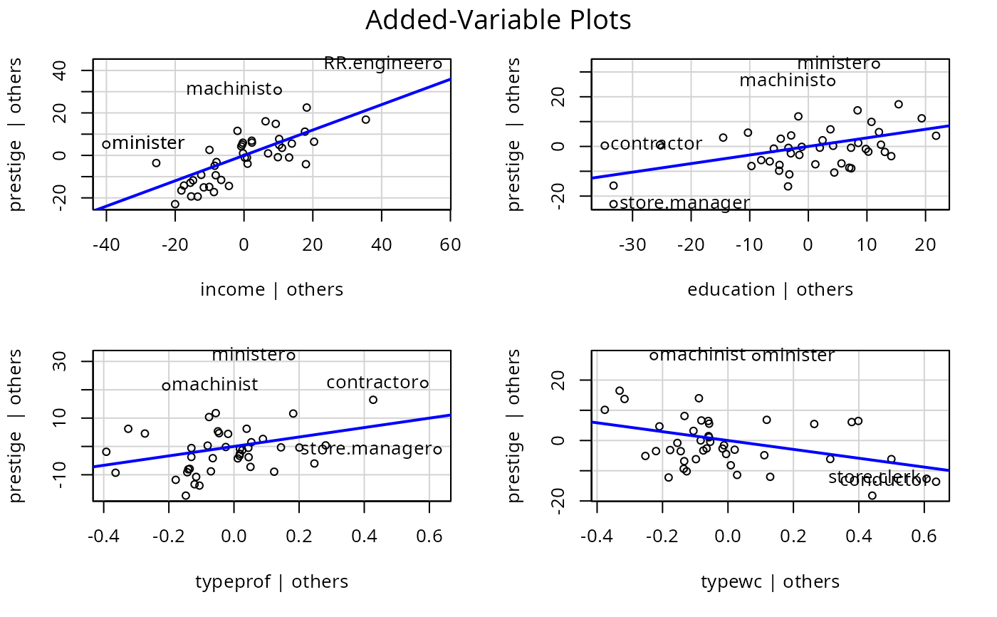
avPlots(lm(prestige ~ income + education + type, data=Duncan))


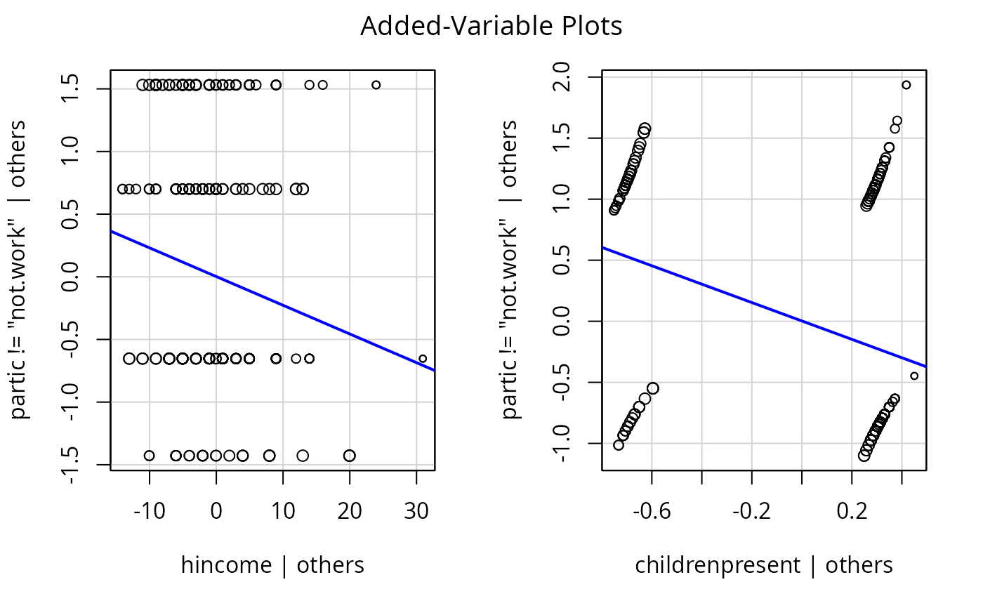
avPlots(glm(partic != "not.work" ~ hincome + children, 
  data=Womenlf, family=binomial), id=FALSE, pt.wts=TRUE)

  
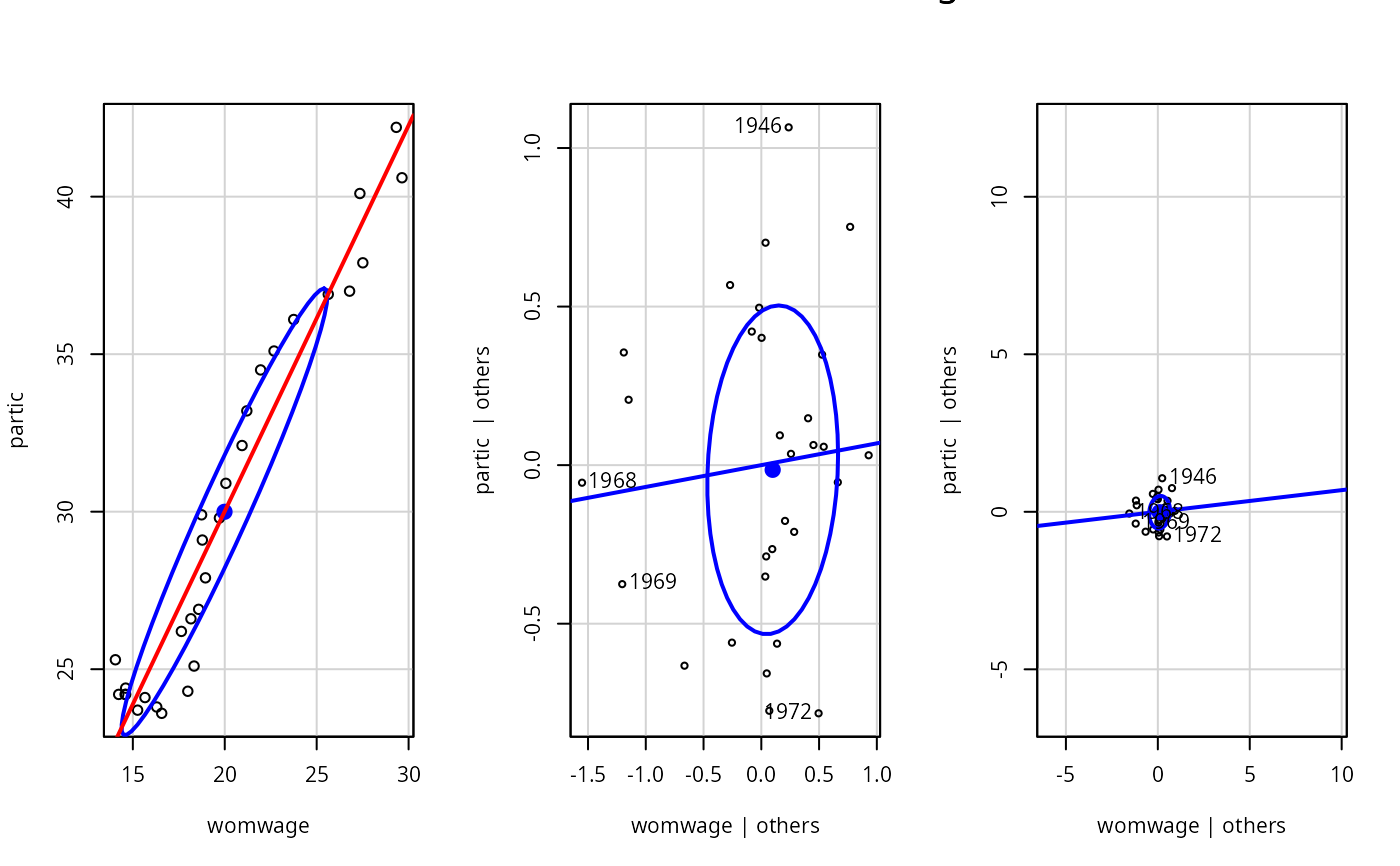
m1 <- lm(partic ~ tfr + menwage + womwage + debt + parttime, Bfox)
par(mfrow=c(1,3))
# marginal plot, ignoring other predictors:
with(Bfox, dataEllipse(womwage, partic, levels=0.5)) 
abline(lm(partic ~ womwage, Bfox), col="red", lwd=2)
# AV plot, adjusting for others:
avPlots(m1, ~ womwage, ellipse=list(levels=0.5)) 
# AV plot, adjusting and scaling as in marginal plot
avPlots(m1, ~ womwage, marginal.scale=TRUE, ellipse=list(levels=0.5)) 


# 3D AV plot, requires the rgl package
if (interactive() && require("rgl")){
avPlot3d(lm(prestige ~ income + education + type, data=Duncan), 
  "income", "education")
}