Component+Residual (Partial Residual) Plots

These functions construct component+residual plots, also called partial-residual plots, for linear and generalized linear models.

Usage

crPlots(model, ...)

# Default S3 method
crPlots(model, terms = ~., layout = NULL, ask, main, 
    ...)

crp(...)

crPlot(model, ...)

# S3 method for class 'lm'
crPlot(model, variable, id=FALSE,
    order=1, line=TRUE, smooth=TRUE, 
    col=carPalette()[1], col.lines=carPalette()[-1],
    xlab, ylab, pch=1, lwd=2, grid=TRUE, ...)
    
crPlot3d(model, var1, var2, ...)

# S3 method for class 'lm'
crPlot3d(model, var1, var2,
    xlab = var1,
    ylab = paste0("C+R(", eff$response, ")"), zlab = var2,
    axis.scales = TRUE, axis.ticks = FALSE, revolutions = 0,
    bg.col = c("white", "black"),
    axis.col = if (bg.col == "white") c("darkmagenta", "black", "darkcyan") 
        else c("darkmagenta", "white", "darkcyan"),
    surface.col = carPalette()[2:3], surface.alpha = 0.5,
    point.col = "yellow", text.col = axis.col,
    grid.col = if (bg.col ==  "white") "black" else "gray",
    fogtype = c("exp2", "linear", "exp", "none"),
    fill = TRUE, grid = TRUE, grid.lines = 26,
    smoother = c("loess", "mgcv", "none"), df.mgcv = NULL, loess.args = NULL,
    sphere.size = 1, radius = 1, threshold = 0.01, speed = 1, fov = 60,
    ellipsoid = FALSE, level = 0.5, ellipsoid.alpha = 0.1,
    id = FALSE, 
    mouseMode=c(none="none", left="polar", right="zoom", middle="fov", 
                 wheel="pull"),
    ...)

Arguments

model: model object produced by lm or glm.
terms: A one-sided formula that specifies a subset of the regressors. One component-plus-residual plot is drawn for each regressor. The default ~. is to plot against all numeric regressors. For example, the specification terms = ~ . - X3 would plot against all regressors except for X3, while terms = ~ log(X4) would give the plot for the predictor X4 that is represented in the model by log(X4). If this argument is a quoted name of one of the predictors, the component-plus-residual plot is drawn for that predictor only.
var1, var2: The quoted names of the two predictors in the model to use for a 3D C+R plot.
layout: If set to a value like c(1, 1) or c(4, 3), the layout of the graph will have this many rows and columns. If not set, the program will select an appropriate layout. If the number of graphs exceed nine, you must select the layout yourself, or you will get a maximum of nine per page. If layout=NA, the function does not set the layout and the user can use the par function to control the layout, for example to have plots from two models in the same graphics window.
ask: If TRUE, ask the user before drawing the next plot; if FALSE, the default, don't ask. This is relevant only if not all the graphs can be drawn in one window.
main: The title of the plot; if missing, one will be supplied.
...: crPlots passes these arguments to crPlot. crPlot passes them to plot.
variable: A quoted string giving the name of a variable for the horizontal axis.
id: controls point identification; if FALSE (the default), no points are identified; can be a list of named arguments to the showLabels function; TRUE is equivalent to list(method=list(abs(residuals(model, type="pearson")), "x"), n=2, cex=1, col=carPalette()[1], location="lr"), which identifies the 2 points with the largest residuals and the 2 points with the most extreme horizontal (X) values. For 3D C+R plots, see Identify3d.
order: order of polynomial regression performed for predictor to be plotted; default 1.
line: TRUE to plot least-squares line.
smooth: specifies the smoother to be used along with its arguments; if FALSE, no smoother is shown; can be a list giving the smoother function and its named arguments; TRUE, the default, is equivalent to list(smoother=loessLine). See ScatterplotSmoothers for the smoothers supplied by the car package and their arguments.
smoother, df.mgcv, loess.args: smoother specifies quoted name of the surface smoother to use for the partial residuals, either loess, the default, or mgcv. df.mgcv gives the degrees of freedom for the mgcv smoother; NULL, the default, causes the df to be computed by mgcv. loess.args is an optional list with named elements span, family and degree, with default span = 2/3; family = "gaussian" for a binomial or Poisson GLM and family = "symmetric" otherwise; and degree = 1 (see loess).
col: color for points; the default is the first entry in the current car palette (see carPalette and par).
col.lines: a list of at least two colors. The first color is used for the ls line and the second color is used for the fitted lowess line. To use the same color for both, use, for example, col.lines=c("red", "red")
xlab, ylab, zlab: labels for the x and y axes, and for the z axis of a 3D plot. If not set appropriate labels are created by the function. for the 3D C+R plot, the predictors are on the x and z axes and the response on the y (vertical) axis.
pch: plotting character for points; default is 1 (a circle, see par).
lwd: line width; default is 2 (see par).
grid: If TRUE, the default, a light-gray background grid is put on the graph. For a 3D C+R plot, see the grid argument for scatter3d.
grid.lines: number of horizontal and vertical lines to be drawn on regression surfaces for 2D C+R plots (26 by default); the square of grid.lines corresponds to the number of points at which the fitted partial regression surface is evaluated and so this argument should not be set too small.
axis.scales, axis.ticks, revolutions, bg.col, axis.col, surface.col, surface.alpha, point.col, text.col, grid.col, fogtype, fill, sphere.size, radius, threshold, speed, fov, ellipsoid, level, ellipsoid.alpha, mouseMode: see scatter3d.

Details

The functions intended for direct use are crPlots, for which crp is an abbreviation, and, for 3D C+R plots, crPlot3d.

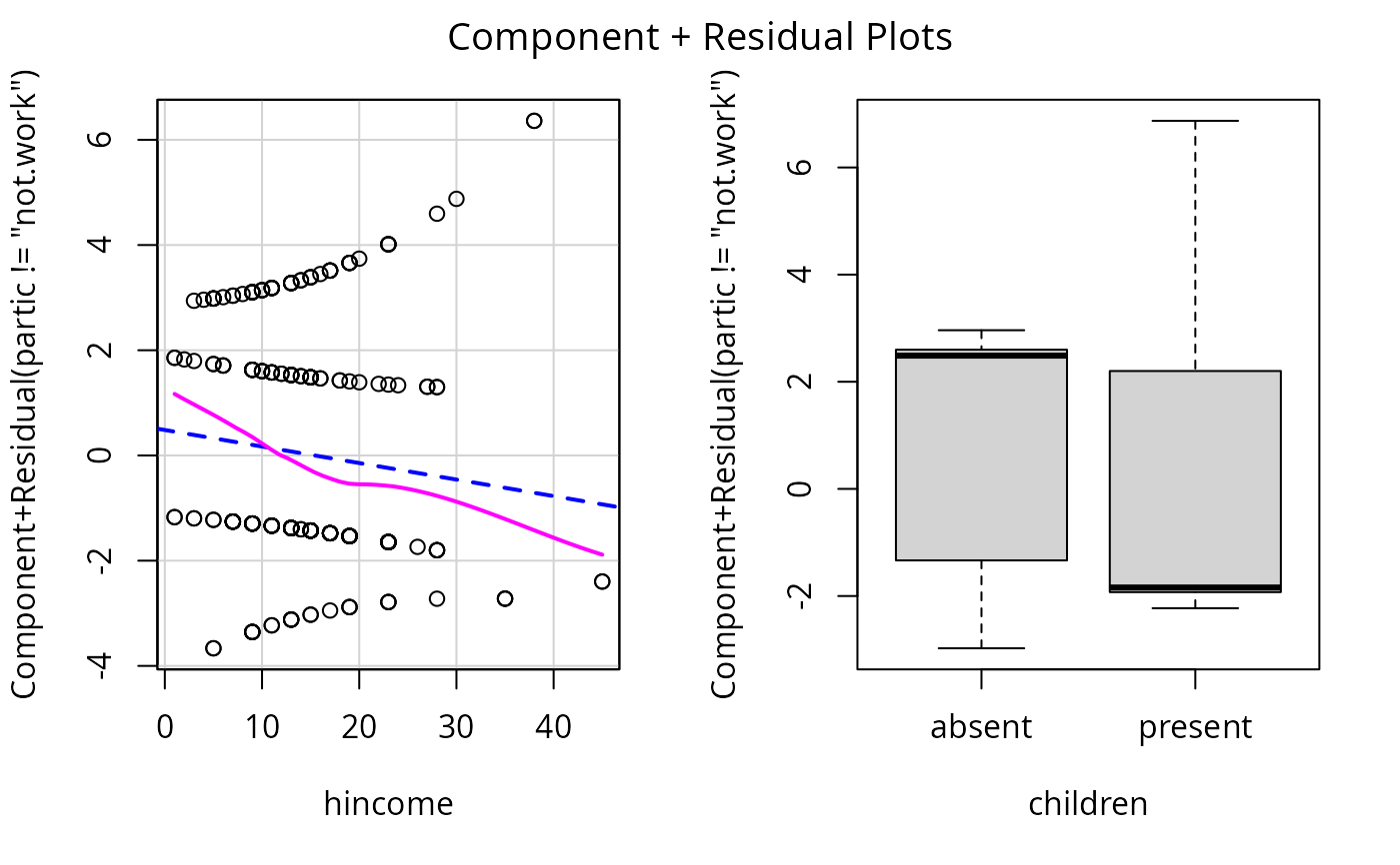
For 2D plots, the model cannot contain interactions, but can contain factors. Parallel boxplots of the partial residuals are drawn for the levels of a factor. crPlot3d can handle models with two-way interactions.

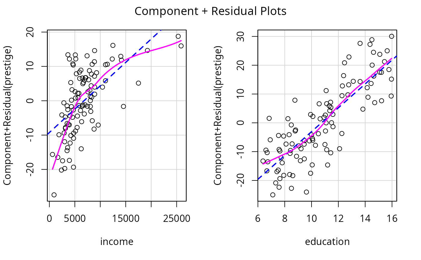
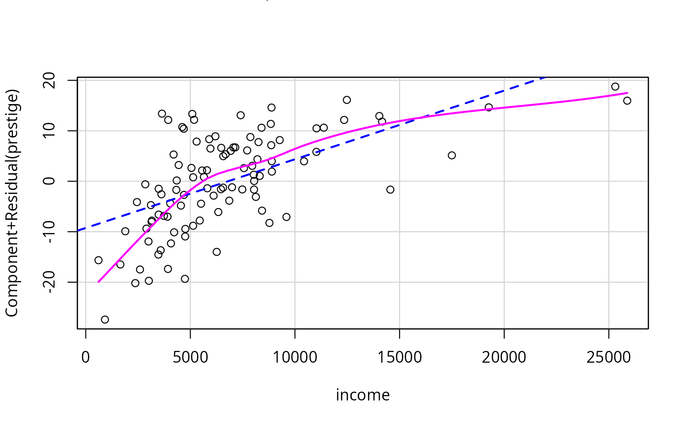
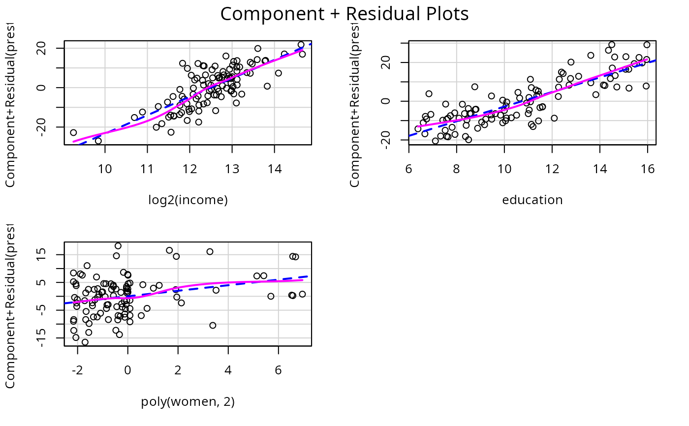
For 2D C+R plots, the fit is represented by a broken blue line and a smooth of the partial residuals by a solid magenta line. For 3D C+R plots, the fit is represented by a blue surface and a smooth of the partial residuals by a magenta surface.

Value

These functions are used for their side effect of producing plots, but also invisibly return the coordinates of the plotted points.

References

Cook, R. D. and Weisberg, S. (1999) Applied Regression, Including Computing and Graphics. Wiley.

Fox, J. (2016) Applied Regression Analysis and Generalized Linear Models, Third Edition. Sage.

Fox, J. and Weisberg, S. (2019) An R Companion to Applied Regression, Third Edition, Sage.

Author

John Fox jfox@mcmaster.ca

Examples

crPlots(m<-lm(prestige ~ income + education, data=Prestige)) 


crPlots(m, terms=~ . - education) # get only one plot


crPlots(lm(prestige ~ log2(income) + education + poly(women,2), data=Prestige))


crPlots(glm(partic != "not.work" ~ hincome + children, 
  data=Womenlf, family=binomial), smooth=list(span=0.75))


# 3D C+R plot, requires the rgl, effects, and mgcv packages
if (interactive() && require(rgl) && require(effects) && require(mgcv)){
crPlot3d(lm(prestige ~ income*education + women, data=Prestige), 
    "income", "education") 
}