Residual Plots for Linear and Generalized Linear Models
residualPlots.RdDraws a plot or plots of residuals versus one or more term in a mean function and/or versus fitted values. For linear models curvature tests are computed for each of the plots by adding a quadratic term to the regression function and testing the quadratic to be zero. This is Tukey's test for nonadditivity when plotting against fitted values.
Usage
### This is a generic function with only one required argument:

residualPlots (model, ...)

# Default S3 method
residualPlots(model, terms= ~ . ,
            layout=NULL, ask, main="",
            fitted=TRUE, AsIs=TRUE, plot=TRUE, tests=TRUE, groups, ...)

# S3 method for class 'lm'
residualPlots(model, ...)

# S3 method for class 'glm'
residualPlots(model, ...)

### residualPlots calls residualPlot, so these arguments can be
### used with either function

residualPlot(model, ...)

# Default S3 method
residualPlot(model, variable = "fitted", type = "pearson",
     groups, plot = TRUE, linear = TRUE,
     quadratic = if(missing(groups)) TRUE else FALSE,
     smooth=FALSE, id=FALSE,
     col = carPalette()[1], col.quad = carPalette()[2], pch=1,
     xlab, ylab, lwd=1, grid=TRUE, key=!missing(groups), ...)

# S3 method for class 'lm'
residualPlot(model, ...)

# S3 method for class 'glm'
residualPlot(model, variable = "fitted", type = "pearson",
    plot = TRUE, quadratic = FALSE, smooth=TRUE, ...)
Arguments
- model
A regression object.
- terms
A one-sided formula that specifies a subset of the terms that appear in the formula that defined the model. The default
~ .is to plot against all first-order terms. Interactions are skipped. For example, the specificationterms = ~ . - X3would plot against all terms except forX3. To get a plot against fitted values only, use the argumentsterms = ~ 1. If a term likelog(X1)is in the formula, then the corresponding plot is obtained usingterms = ~ log(X1). For polynomial terms generated using thepolyfunction, the plot is against the first-order variable, which may be centered and scaled depending on how the arguments to thepolyfunction. Plots against factors are boxplots. Plots against splines use the result ofpredict(model), type="terms")[, variable])as the horizontal axis.A grouping variable can also be specified, so, for example
terms= ~ .|typewould use the factortypeto set a different color and symbol for each level oftype. Any fits in the plots will also be done separately for each level of group. This can be useful of finding interactions between the grouping variable and the term on the horizontal axis. The grouping variable can also be set using the argumentgoups="type".- layout
If set to a value like
c(1, 1)orc(4, 3), the layout of the graph will have this many rows and columns per "page" with a prompt given the in console to change to the next page. If not set, the program will select an appropriate layout. If the number of graphs exceed nine, you must select the layout yourself, or you will get a maximum of nine per page. Iflayout=NA, the function does not set the layout and the user can use theparfunction to control the layout, for example to have plots from two models in the same graphics window.- ask
If
TRUE, ask the user before drawing the next plot; ifFALSE, don't ask.- main
Main title for the graphs. The default is
main=""for no title.- fitted
If
TRUE, the default, include the plot against fitted values.- AsIs
Some terms in a model formula use the as-is or identity function, for example a term like
I(X^2)to include a quadratic. These terms will be skipped in plotting ifAsIsisFALSE. The default isTRUE.- plot
If
TRUE, draw the plot(s).- tests
If
TRUE, display the curvature tests.- ...
Additional arguments passed to
residualPlotand then toplot.- variable
Quoted variable name for the factor or regressor to be put on the horizontal axis, or the default
"fitted"to plot versus fitted values.- type
Specifies the type of residual to be plotted. Any of
c("working", "response", "deviance", "pearson", "partial", "rstudent", "rstandard")may be specified. The defaulttype = "pearson"is usually appropriate, since it is equal to ordinary residuals observed minus fit with ols, and correctly weighted residuals with wls or for a glm. The last two options use therstudentandrstandardfunctions and use studentized or standardized residuals.- groups
A grouping indicator, provided as the quoted name of a grouping variable in the model, such as "type", or "ageGroup". Points in different groups will be plotted with different colors and symbols. If missing, no grouping is used. In
residualPlots, the grouping variable can also be set in thetermsargument, as described above. The default is no grouping.- linear
If
TRUE, adds a horizontal line at zero if no groups. With groups, within level of groups display the ols regression of the residuals as response and the horizontal axis as the regressor.- quadratic
if
TRUE, fits the quadratic regression of the vertical axis on the horizontal axis and displays a lack of fit test. Default isTRUEforlmandFALSEforglmor ifgroupsnot missing.- smooth
specifies the smoother to be used along with its arguments; if
FALSE, which is the default except for generalized linear models, no smoother is shown; can be a list giving the smoother function and its named arguments;TRUEis equivalent tolist(smoother=loessLine, span=2/3, col=carPalette()[3]), which is the default for a GLM. SeeScatterplotSmoothersfor the smoothers supplied by the car package and their arguments.- id
controls point identification; if
FALSE(the default), no points are identified; can be a list of named arguments to theshowLabelsfunction;TRUEis equivalent tolist(method="r", n=2, cex=1, col=carPalette()[1], location="lr"), which identifies the 2 points with the largest absolute residuals.- col
default color for points. If groups is set, col can be a list at least as long as the number of levels for groups giving the colors for each groups.
- col.quad
default color for quadratic fit if groups is missing. Ignored if groups are used.
- pch
plotting character. The default is pch=1. If groups are used, pch can be set to a vector at least as long as the number of groups.
- xlab
X-axis label. If not specified, a useful label is constructed by the function.
- ylab
Y-axis label. If not specified, a useful label is constructed by the function.
- lwd
line width for the quadratic fit, if any.
- grid
If TRUE, the default, a light-gray background grid is put on the graph
- key
Should a key be added to the plot? Default is
!is.null(groups).
Details
residualPlots draws one or more residuals plots depending on the
value of the terms and fitted arguments. If terms = ~ .,
the default, then a plot is produced of residuals versus each first-order
term in the formula used to create the model. A plot of
residuals versus fitted values is also included unless fitted=FALSE. Setting terms = ~1
will provide only the plot against fitted values.
A table of curvature tests is displayed for linear models. For plots
against a term in the model formula, say X1, the test displayed is
the t-test for for I(X1^2) in the fit of update, model, ~. + I(X1^2)).
Econometricians call this a specification test. For factors, the displayed
plot is a boxplot, no curvature test is computed, and grouping is ignored.
For fitted values in a linear model, the test is Tukey's one-degree-of-freedom test for
nonadditivity. You can suppress the tests with the argument tests=FALSE.
If grouping is used curvature tests are not displayed.
residualPlot, which is called by residualPlots,
should be viewed as an internal function, and is included here to display its
arguments, which can be used with residualPlots as well. The
residualPlot function returns the curvature test as an invisible result.
residCurvTest computes the curvature test only. For any factors a
boxplot will be drawn. For any polynomials, plots are against the linear term.
Other non-standard predictors like B-splines are skipped.
Value
For lm objects,
returns a data.frame with one row for each plot drawn, one column for
the curvature test statistic, and a second column for the corresponding
p-value. This function is used primarily for its side effect of drawing
residual plots.
References
Fox, J. and Weisberg, S. (2019) An R Companion to Applied Regression, Third Edition. Sage.
Weisberg, S. (2014) Applied Linear Regression, Fourth Edition, Wiley, Chapter 8
Author
Sanford Weisberg, sandy@umn.edu
See also
See Also lm, identify,
showLabels
Examples
m1 <- lm(prestige ~ income + type, data=Prestige)
residualPlots(m1)
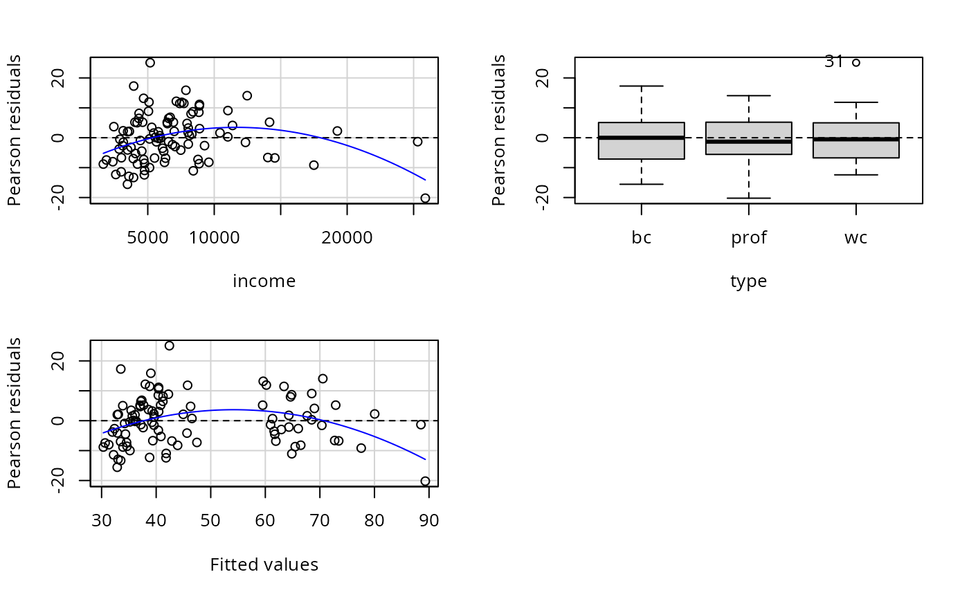 #> Test stat Pr(>|Test stat|)
#> income -3.9175 0.0001707 ***
#> type
#> Tukey test -4.9317 8.153e-07 ***
#> ---
#> Signif. codes: 0 ‘***’ 0.001 ‘**’ 0.01 ‘*’ 0.05 ‘.’ 0.1 ‘ ’ 1
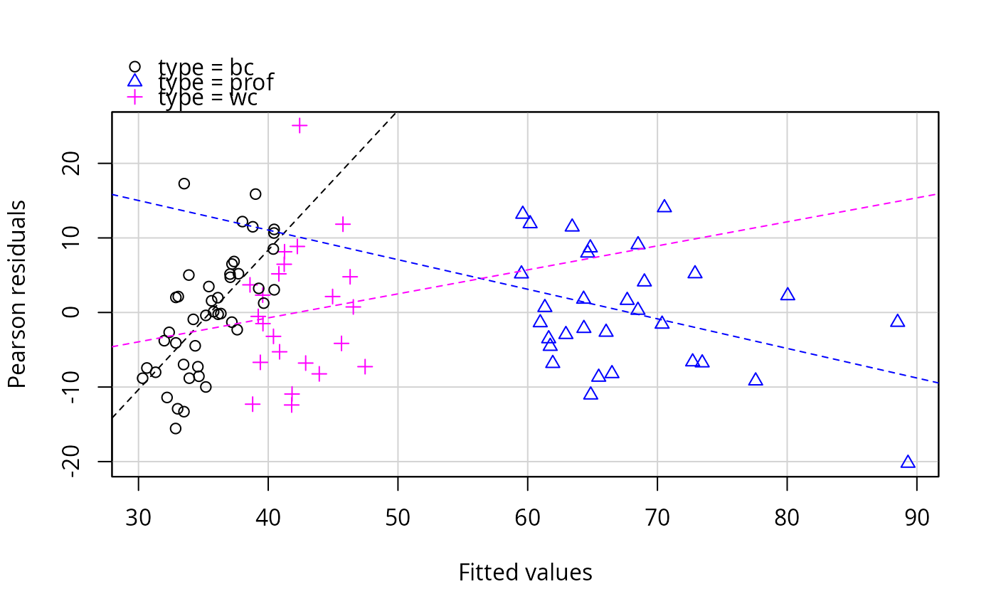
residualPlots(m1, terms= ~ 1 | type) # plot vs. yhat grouping by type
#> Test stat Pr(>|Test stat|)
#> income -3.9175 0.0001707 ***
#> type
#> Tukey test -4.9317 8.153e-07 ***
#> ---
#> Signif. codes: 0 ‘***’ 0.001 ‘**’ 0.01 ‘*’ 0.05 ‘.’ 0.1 ‘ ’ 1
residualPlots(m1, terms= ~ 1 | type) # plot vs. yhat grouping by type