Ceres Plots

These functions draw Ceres plots for linear and generalized linear models.

Usage

ceresPlots(model, ...)

# Default S3 method
ceresPlots(model, terms = ~., layout = NULL, ask, main,
    ...)

ceresPlot(model, ...)

# S3 method for class 'lm'
ceresPlot(model, variable, id=FALSE,
  line=TRUE,  smooth=TRUE, col=carPalette()[1], col.lines=carPalette()[-1],
  xlab, ylab, pch=1, lwd=2,  grid=TRUE, ...)

# S3 method for class 'glm'
ceresPlot(model, ...)

Arguments

model

model object produced by lm or glm.

terms

A one-sided formula that specifies a subset of the regressors. One component-plus-residual plot is drawn for each term. The default ~. is to plot against all numeric predictors. For example, the specification terms = ~ . - X3 would plot against all predictors except for X3. Factors and nonstandard predictors such as B-splines are skipped. If this argument is a quoted name of one of the regressors, the component-plus-residual plot is drawn for that predictor only.

layout

If set to a value like c(1, 1) or c(4, 3), the layout of the graph will have this many rows and columns. If not set, the program will select an appropriate layout. If the number of graphs exceed nine, you must select the layout yourself, or you will get a maximum of nine per page. If layout=NA, the function does not set the layout and the user can use the par function to control the layout, for example to have plots from two models in the same graphics window.

ask

If TRUE, ask the user before drawing the next plot; if FALSE, the default, don't ask. This is relevant only if not all the graphs can be drawn in one window.

main

Overall title for any array of cerers plots; if missing a default is provided.

...

ceresPlots passes these arguments to ceresPlot. ceresPlot passes them to plot.

variable

A quoted string giving the name of a variable for the horizontal axis

id

controls point identification; if FALSE (the default), no points are identified; can be a list of named arguments to the showLabels function; TRUE is equivalent to list(method=list(abs(residuals(model, type="pearson")), "x"), n=2, cex=1, col=carPalette()[1], location="lr"), which identifies the 2 points with the largest residuals and the 2 points with the most extreme horizontal (X) values.

line

TRUE to plot least-squares line.

smooth

specifies the smoother to be used along with its arguments; if FALSE, no smoother is shown; can be a list giving the smoother function and its named arguments; TRUE, the default, is equivalent to list(smoother=loessLine). See ScatterplotSmoothers for the smoothers supplied by the car package and their arguments. Ceres plots do not support variance smooths.

col

color for points; the default is the first entry in the current car palette (see carPalette and par).

col.lines

a list of at least two colors. The first color is used for the ls line and the second color is used for the fitted lowess line. To use the same color for both, use, for example, col.lines=c("red", "red")

xlab,ylab

labels for the x and y axes, respectively. If not set appropriate labels are created by the function.

pch

plotting character for points; default is 1 (a circle, see par).

lwd

line width; default is 2 (see par).

grid

If TRUE, the default, a light-gray background grid is put on the graph

Details

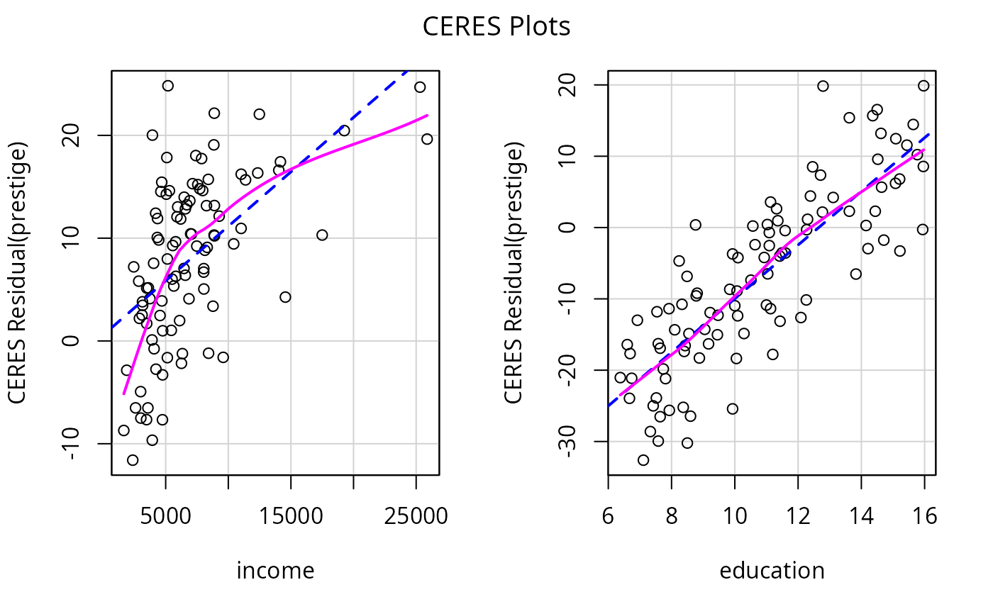
Ceres plots are a generalization of component+residual (partial residual) plots that are less prone to leakage of nonlinearity among the predictors.

The function intended for direct use is ceresPlots.

The model cannot contain interactions, but can contain factors. Factors may be present in the model, but Ceres plots cannot be drawn for them.

Value

NULL. These functions are used for their side effect: producing plots.

References

Cook, R. D. and Weisberg, S. (1999) Applied Regression, Including Computing and Graphics. Wiley.

Fox, J. (2016) Applied Regression Analysis and Generalized Linear Models, Third Edition. Sage.

Fox, J. and Weisberg, S. (2019) An R Companion to Applied Regression, Third Edition, Sage.

Author

John Fox jfox@mcmaster.ca

See also

crPlots, avPlots, showLabels

Examples

ceresPlots(lm(prestige~income+education+type, data=Prestige), terms= ~ . - type)