Summarize Data for Making Tables and Plots

summary.formula summarizes the variables listed in an S formula, computing descriptive statistics (including ones in a user-specified function). The summary statistics may be passed to print methods, plot methods for making annotated dot charts, and latex methods for typesetting tables using LaTeX. summary.formula has three methods for computing descriptive statistics on univariate or multivariate responses, subsetted by categories of other variables. The method of summarization is specified in the parameter method (see details below). For the response and cross methods, the statistics used to summarize the data may be specified in a very flexible way (e.g., the geometric mean, 33rd percentile, Kaplan-Meier 2-year survival estimate, mixtures of several statistics). The default summary statistic for these methods is the mean (the proportion of positive responses for a binary response variable). The cross method is useful for creating data frames which contain summary statistics that are passed to trellis as raw data (to make multi-panel dot charts, for example). The print methods use the print.char.matrix function to print boxed tables.

The right hand side of formula may contain mChoice (“multiple choice”) variables. When test=TRUE each choice is tested separately as a binary categorical response.

The plot method for method="reverse" creates a temporary function Key in frame 0 as is done by the xYplot and Ecdf.formula functions. After plot runs, you can type Key() to put a legend in a default location, or e.g. Key(locator(1)) to draw a legend where you click the left mouse button. This key is for categorical variables, so to have the opportunity to put the key on the graph you will probably want to use the command plot(object, which="categorical"). A second function Key2 is created if continuous variables are being plotted. It is used the same as Key. If the which argument is not specified to plot, two pages of plots will be produced. If you don't define par(mfrow=) yourself, plot.summary.formula.reverse will try to lay out a multi-panel graph to best fit all the individual dot charts for continuous variables.

There is a subscripting method for objects created with method="response". This can be used to print or plot selected variables or summary statistics where there would otherwise be too many on one page.

cumcategory is a utility function useful when summarizing an ordinal response variable. It converts such a variable having k levels to a matrix with k-1 columns, where column i is a vector of zeros and ones indicating that the categorical response is in level i+1 or greater. When the left hand side of formula is cumcategory(y), the default fun will summarize it by computing all of the relevant cumulative proportions.

Functions conTestkw, catTestchisq, ordTestpo are the default statistical test functions for summary.formula. These defaults are: Wilcoxon-Kruskal-Wallis test for continuous variables, Pearson chi-square test for categorical variables, and the likelihood ratio chi-square test from the proportional odds model for ordinal variables. These three functions serve also as templates for the user to create her own testing functions that are self-defining in terms of how the results are printed or rendered in LaTeX, or plotted.

Usage

# S3 method for class 'formula'
summary(formula, data=NULL, subset=NULL,
        na.action=NULL, fun = NULL,
        method = c("response", "reverse", "cross"),
        overall = method == "response" | method == "cross",
        continuous = 10, na.rm = TRUE, na.include = method != "reverse",
        g = 4, quant = c(0.025, 0.05, 0.125, 0.25, 0.375, 0.5, 0.625,
                         0.75, 0.875, 0.95, 0.975),
        nmin = if (method == "reverse") 100
               else 0,
        test = FALSE, conTest = conTestkw, catTest = catTestchisq,
        ordTest = ordTestpo, ...)

# S3 method for class 'summary.formula.response'
x[i, j, drop = FALSE]

# S3 method for class 'summary.formula.response'
print(x, vnames=c('labels','names'), prUnits=TRUE,
      abbreviate.dimnames=FALSE,
      prefix.width, min.colwidth, formatArgs=NULL, markdown=FALSE, ...)

# S3 method for class 'summary.formula.response'
plot(x, which = 1, vnames = c('labels','names'), xlim, xlab,
     pch = c(16, 1, 2, 17, 15, 3, 4, 5, 0), superposeStrata = TRUE,
     dotfont = 1, add = FALSE, reset.par = TRUE, main, subtitles = TRUE,
     ...)

# S3 method for class 'summary.formula.response'
latex(object, title = first.word(deparse(substitute(object))), caption,
      trios, vnames = c('labels', 'names'), prn = TRUE, prUnits = TRUE,
      rowlabel = '', cdec = 2, ncaption = TRUE, ...)

# S3 method for class 'summary.formula.reverse'
print(x, digits, prn = any(n != N), pctdig = 0,
      what=c('%', 'proportion'),
      npct = c('numerator', 'both', 'denominator', 'none'),
      exclude1 = TRUE, vnames = c('labels', 'names'), prUnits = TRUE,
      sep = '/', abbreviate.dimnames = FALSE,
      prefix.width = max(nchar(lab)), min.colwidth, formatArgs=NULL, round=NULL,
      prtest = c('P','stat','df','name'), prmsd = FALSE, long = FALSE,
      pdig = 3, eps = 0.001, ...)

# S3 method for class 'summary.formula.reverse'
plot(x, vnames = c('labels', 'names'), what = c('proportion', '%'),
     which = c('both', 'categorical', 'continuous'),
     xlim = if(what == 'proportion') c(0,1)
            else c(0,100), 
     xlab = if(what=='proportion') 'Proportion'
            else 'Percentage', 
     pch = c(16, 1, 2, 17, 15, 3, 4, 5, 0), exclude1 = TRUE,
     dotfont = 1, main,
     prtest = c('P', 'stat', 'df', 'name'), pdig = 3, eps = 0.001,
     conType = c('dot', 'bp', 'raw'), cex.means = 0.5, ...)

# S3 method for class 'summary.formula.reverse'
latex(object, title = first.word(deparse(substitute(object))), digits,
      prn = any(n != N), pctdig = 0, what=c('%', 'proportion'),
      npct = c("numerator", "both", "denominator", "slash", "none"),
      npct.size = 'scriptsize', Nsize = "scriptsize", exclude1 = TRUE,
      vnames=c("labels", "names"), prUnits = TRUE, middle.bold = FALSE,
      outer.size = "scriptsize", caption, rowlabel = "",
      insert.bottom = TRUE, dcolumn = FALSE, formatArgs=NULL, round = NULL,
      prtest = c('P', 'stat', 'df', 'name'), prmsd = FALSE,
      msdsize = NULL, long = dotchart, pdig = 3, eps = 0.001,
      auxCol = NULL, dotchart=FALSE, ...)

# S3 method for class 'summary.formula.cross'
print(x, twoway = nvar == 2, prnmiss = any(stats$Missing > 0), prn = TRUE,
      abbreviate.dimnames = FALSE, prefix.width = max(nchar(v)),
      min.colwidth, formatArgs = NULL, ...)

# S3 method for class 'summary.formula.cross'
latex(object, title = first.word(deparse(substitute(object))),
      twoway = nvar == 2, prnmiss = TRUE, prn = TRUE,
      caption=attr(object, "heading"), vnames=c("labels", "names"),
      rowlabel="", ...)

stratify(..., na.group = FALSE, shortlabel = TRUE)

# S3 method for class 'summary.formula.cross'
formula(x, ...)

cumcategory(y)

conTestkw(group, x)
catTestchisq(tab)
ordTestpo(group, x)

Arguments

formula

An R formula with additive effects. For method="response" or "cross", the dependent variable has the usual connotation. For method="reverse", the dependent variable is what is usually thought of as an independent variable, and it is one that is used to stratify all of the right hand side variables. For method="response" (only), the formula may contain one or more invocations of the stratify function whose arguments are defined below. This causes the entire analysis to be stratified by cross-classifications of the combined list of stratification factors. This stratification will be reflected as major column groupings in the resulting table, or as more response columns for plotting. If formula has no dependent variable method="reverse" is the only legal value and so method defaults to "reverse" in this case.

x

an object created by summary.formula. For conTestkw a numeric vector, and for ordTestpo, a numeric or factor variable that can be considered ordered

y

a numeric, character, category, or factor vector for cumcategory. Is converted to a categorical variable is needed.

drop

logical. If TRUE the result is coerced to the lowest possible dimension.

data

name or number of a data frame. Default is the current frame.

subset

a logical vector or integer vector of subscripts used to specify the subset of data to use in the analysis. The default is to use all observations in the data frame.

na.action

function for handling missing data in the input data. The default is a function defined here called na.retain, which keeps all observations for processing, with missing variables or not.

fun

function for summarizing data in each cell. Default is to take the mean of each column of the possibly multivariate response variable. You can specify fun="%" to compute percentages (100 times the mean of a series of logical or binary variables). User–specified functions can also return a matrix. For example, you might compute quartiles on a bivariate response. Does not apply to method="reverse".

method

The default is "response", in which case the response variable may be multivariate and any number of statistics may be used to summarize them. Here the responses are summarized separately for each of any number of independent variables. Continuous independent variables (see the continuous parameter below) are automatically stratified into g (see below) quantile groups (if you want to control the discretization for selected variables, use the cut2 function on them). Otherwise, the data are subsetted by all levels of discrete right hand side variables. For multivariate responses, subjects are considered to be missing if any of the columns is missing.

The method="reverse" option is typically used to make baseline characteristic tables, for example. The single left hand side variable must be categorical (e.g., treatment), and the right hand side variables are broken down one at a time by the "dependent" variable. Continuous variables are described by three quantiles (quartiles by default) along with outer quantiles (used only for scaling x-axes when plotting quartiles; all are used when plotting box-percentile plots), and categorical ones are described by counts and percentages. If there is no left hand side variable, summary assumes that there is only one group in the data, so that only one column of summaries will appear. If there is no dependent variable in formula, method defaults to "reverse" automatically.

The method="cross" option allows for a multivariate dependent variable and for up to three independents. Continuous independent variables (those with at least continuous unique values) are automatically divided into g quantile groups. The independents are cross-classified, and marginal statistics may optionally be computed. The output of summary.formula in this case is a data frame containing the independent variable combinations (with levels of "All" corresponding to marginals) and the corresponding summary statistics in the matrix S. The output data frame is suitable for direct use in trellis. The print and latex typesetting methods for this method allows for a special two-way format if there are two right hand variables.

overall

For method="reverse", setting overall=TRUE makes a new column with overall statistics for the whole sample. For method="cross", overall=TRUE (the default) results in all marginal statistics being computed. For trellis displays (usually multi-panel dot plots), these marginals just form other categories. For "response", the default is overall=TRUE, causing a final row of global summary statistics to appear in tables and dot charts. If test=TRUE these marginal statistics are ignored in doing statistical tests.

continuous

specifies the threshold for when a variable is considered to be continuous (when there are at least continuous unique values). factor variables are always considered to be categorical no matter how many levels they have.

na.rm

TRUE (the default) to exclude NAs before passing data to fun to compute statistics, FALSE otherwise. na.rm=FALSE is useful if the response variable is a matrix and you do not wish to exclude a row of the matrix if any of the columns in that row are NA. na.rm also applies to summary statistic functions such as smean.cl.normal. For these na.rm defaults to TRUE unlike built-in functions.

na.include

for method="response", set na.include=FALSE to exclude missing values from being counted as their own category when subsetting the response(s) by levels of a categorical variable. For method="reverse" set na.include=TRUE to keep missing values of categorical variables from being excluded from the table.

g

number of quantile groups to use when variables are automatically categorized with method="response" or "cross" using cut2

nmin

if fewer than nmin observations exist in a category for "response" (over all strata combined), that category will be ignored. For "reverse", for categories of the response variable in which there are less than or equal to nmin non-missing observations, the raw data are retained for later plotting in place of box plots.

test

applies if method="reverse". Set to TRUE to compute test statistics using tests specified in conTest and catTest.

conTest

a function of two arguments (grouping variable and a continuous variable) that returns a list with components P (the computed P-value), stat (the test statistic, either chi-square or F), df (degrees of freedom), testname (test name), statname (statistic name), namefun ("chisq", "fstat"), an optional component latexstat (LaTeX representation of statname), an optional component plotmathstat (for R - the plotmath representation of statname, as a character string), and an optional component note that contains a character string note about the test (e.g., "test not done because n < 5"). conTest is applied to continuous variables on the right-hand-side of the formula when method="reverse". The default uses the spearman2 function to run the Wilcoxon or Kruskal-Wallis test using the F distribution.

catTest

a function of a frequency table (an integer matrix) that returns a list with the same components as created by conTest. By default, the Pearson chi-square test is done, without continuity correction (the continuity correction would make the test conservative like the Fisher exact test).

ordTest

a function of a frequency table (an integer matrix) that returns a list with the same components as created by conTest. By default, the Proportional odds likelihood ratio test is done.

...

for summary.formula these are optional arguments for cut2 when variables are automatically categorized. For plot methods these arguments are passed to dotchart2. For Key and Key2 these arguments are passed to key, text, or mtitle. For print methods these are optional arguments to print.char.matrix. For latex methods these are passed to latex.default. One of the most important of these is file. Specifying file="" will cause LaTeX code to just be printed to standard output rather than be stored in a permanent file.

object

an object created by summary.formula

quant

vector of quantiles to use for summarizing data with method="reverse". This must be numbers between 0 and 1 inclusive and must include the numbers 0.5, 0.25, and 0.75 which are used for printing and for plotting quantile intervals. The outer quantiles are used for scaling the x-axes for such plots. Specify outer quantiles as 0 and 1 to scale the x-axes using the whole observed data ranges instead of the default (a 0.95 quantile interval). Box-percentile plots are drawn using all but the outer quantiles.

vnames

By default, tables and plots are usually labeled with variable labels (see the label and sas.get functions). To use the shorter variable names, specify vnames="name".

pch

vector of plotting characters to represent different groups, in order of group levels. For method="response" the characters correspond to levels of the stratify variable if superposeStrata=TRUE, and if no strata are used or if superposeStrata=FALSE, the pch vector corresponds to the which argument for method="response".

superposeStrata

If stratify was used, set superposeStrata=FALSE to make separate dot charts for each level of the stratification variable, for method='response'. The default is to superposition all strata on one dot chart.

dotfont

font for plotting points

reset.par

set to FALSE to suppress the restoring of the old par values in plot.summary.formula.response

abbreviate.dimnames

see print.char.matrix

prefix.width

see print.char.matrix

min.colwidth

minimum column width to use for boxes printed with print.char.matrix. The default is the maximum of the minimum column label length and the minimum length of entries in the data cells.

formatArgs

a list containing other arguments to pass to format.default such as scientific, e.g., formatArgs=list(scientific=c(-5,5)). For print.summary.formula.reverse and format.summary.formula.reverse, formatArgs applies only to statistics computed on continuous variables, not to percents, numerators, and denominators. The round argument may be preferred.

markdown

for print.summary.formula.response set to TRUE to use knitr::kable to produce the table in markdown format rather than using raw text output created by print.char.matrix

digits

number of significant digits to print. Default is to use the current value of the digits system option.

prn

set to TRUE to print the number of non-missing observations on the current (row) variable. The default is to print these only if any of the counts of non-missing values differs from the total number of non-missing values of the left-hand-side variable. For method="cross" the default is to always print N.

prnmiss

set to FALSE to suppress printing counts of missing values for "cross"

what

for method="reverse" specifies whether proportions or percentages are to be plotted

pctdig

number of digits to the right of the decimal place for printing percentages. The default is zero, so percents will be rounded to the nearest percent.

npct

specifies which counts are to be printed to the right of percentages. The default is to print the frequency (numerator of the percent) in parentheses. You can specify "both" to print both numerator and denominator, "denominator", "slash" to typeset horizontally using a forward slash, or "none".

npct.size

the size for typesetting npct information which appears after percents. The default is "scriptsize".

Nsize

When a second row of column headings is added showing sample sizes, Nsize specifies the LaTeX size for these subheadings. Default is "scriptsize".

exclude1

by default, method="reverse" objects will be printed, plotted, or typeset by removing redundant entries from percentage tables for categorical variables. For example, if you print the percent of females, you don't need to print the percent of males. To override this, set exclude1=FALSE.

prUnits

set to FALSE to suppress printing or latexing units attributes of variables, when method='reverse' or 'response'

sep

character to use to separate quantiles when printing method="reverse" tables

prtest

a vector of test statistic components to print if test=TRUE was in effect when summary.formula was called. Defaults to printing all components. Specify prtest=FALSE or prtest="none" to not print any tests. This applies to print, latex, and plot methods for method='reverse'.

round

for print.summary.formula.reverse and latex.summary.formula.reverse specify round to round the quantiles and optional mean and standard deviation to round digits after the decimal point

prmsd

set to TRUE to print mean and SD after the three quantiles, for continuous variables with method="reverse"

msdsize

defaults to NULL to use the current font size for the mean and standard deviation if prmsd is TRUE. Set to a character string to specify an alternate LaTeX font size.

long

set to TRUE to print the results for the first category on its own line, not on the same line with the variable label (for method="reverse" with print and latex methods)

pdig

number of digits to the right of the decimal place for printing P-values. Default is 3. This is passed to format.pval.

eps

P-values less than eps will be printed as < eps. See format.pval.

auxCol

an optional auxiliary column of information, right justified, to add in front of statistics typeset by latex.summary.formula.reverse. This argument is a list with a single element that has a name specifying the column heading. If this name includes a newline character, the portions of the string before and after the newline form respectively the main heading and the subheading (typically set in smaller font), respectively. See the extracolheads argument to latex.default. auxCol is filled with blanks when a variable being summarized takes up more than one row in the output. This happens with categorical variables.

twoway

for method="cross" with two right hand side variables, twoway controls whether the resulting table will be printed in enumeration format or as a two-way table (the default)

which

For method="response" specifies the sequential number or a vector of subscripts of statistics to plot. If you had any stratify variables, these are counted as if more statistics were computed. For method="reverse" specifies whether to plot results for categorical variables, continuous variables, or both (the default).

conType

For plotting method="reverse" plots for continuous variables, dot plots showing quartiles are drawn by default. Specify conType='bp' to draw box-percentile plots using all the quantiles in quant except the outermost ones. Means are drawn with a solid dot and vertical reference lines are placed at the three quartiles. Specify conType='raw' to make a strip chart showing the raw data. This can only be used if the sample size for each left-hand-side group is less than or equal to nmin.

cex.means

character size for means in box-percentile plots; default is .5

xlim

vector of length two specifying x-axis limits. For method="reverse", this is only used for plotting categorical variables. Limits for continuous variables are determined by the outer quantiles specified in quant.

xlab

x-axis label

add

set to TRUE to add to an existing plot

main

a main title. For method="reverse" this applies only to the plot for categorical variables.

subtitles

set to FALSE to suppress automatic subtitles

caption

character string containing LaTeX table captions.

title

name of resulting LaTeX file omitting the .tex suffix. Default is the name of the summary object. If caption is specied, title is also used for the table's symbolic reference label.

trios

If for method="response" you summarized the response(s) by using three quantiles, specify trios=TRUE or trios=v to group each set of three statistics into one column for latex output, using the format a B c, where the outer quantiles are in smaller font (scriptsize). For trios=TRUE, the overall column names are taken from the column names of the original data matrix. To give new column names, specify trios=v, where v is a vector of column names, of length m/3, where m is the original number of columns of summary statistics.

rowlabel

see latex.default (under the help file latex)

cdec

number of decimal places to the right of the decimal point for latex. This value should be a scalar (which will be properly replicated), or a vector with length equal to the number of columns in the table. For "response" tables, this length does not count the column for N.

ncaption

set to FALSE to not have latex.summary.formula.response put sample sizes in captions

i

a vector of integers, or character strings containing variable names to subset on. Note that each row subsetted on in an summary.formula.reverse object subsets on all the levels that make up the corresponding variable (automatically).

j

a vector of integers representing column numbers

middle.bold

set to TRUE to have LaTeX use bold face for the middle quantile for method="reverse"

outer.size

the font size for outer quantiles for "reverse" tables

insert.bottom

set to FALSE to suppress inclusion of definitions placed at the bottom of LaTeX tables for method="reverse"

dcolumn

see latex

na.group

set to TRUE to have missing stratification variables given their own category (NA)

shortlabel

set to FALSE to include stratification variable names and equal signs in labels for strata levels

dotchart

set to TRUE to output a dotchart in the latex table being generated.

group

for conTest and ordTest, a numeric or factor variable with length the same as x

tab

for catTest, a frequency table such as that created by table()

Value

summary.formula returns a data frame or list depending on method. plot.summary.formula.reverse returns the number of pages of plots that were made.

Side Effects

plot.summary.formula.reverse creates a function Key and Key2 in frame 0 that will draw legends.

Author

Frank Harrell
Department of Biostatistics
Vanderbilt University
fh@fharrell.com

References

Harrell FE (2007): Statistical tables and plots using S and LaTeX. Document available from https://hbiostat.org/R/Hmisc/summary.pdf.

See also

mChoice, smean.sd, summarize, label, strata, dotchart2, print.char.matrix, update, formula, cut2, llist, format.default, latex, latexTranslate bpplt, summaryM, summary

Examples

options(digits=3)
set.seed(173)
sex <- factor(sample(c("m","f"), 500, rep=TRUE))
age <- rnorm(500, 50, 5)
treatment <- factor(sample(c("Drug","Placebo"), 500, rep=TRUE))

# Generate a 3-choice variable; each of 3 variables has 5 possible levels
symp <- c('Headache','Stomach Ache','Hangnail',
          'Muscle Ache','Depressed')
symptom1 <- sample(symp, 500,TRUE)
symptom2 <- sample(symp, 500,TRUE)
symptom3 <- sample(symp, 500,TRUE)
Symptoms <- mChoice(symptom1, symptom2, symptom3, label='Primary Symptoms')
table(Symptoms)
#> Symptoms
#>     1   1;2 1;2;3 1;2;4 1;2;5   1;3 1;3;4 1;3;5   1;4 1;4;5   1;5     2   2;3 
#>     0     0     0     0     0     0     0     0     0     0     0     0     0 
#> 2;3;4 2;3;5   2;4 2;4;5   2;5     3   3;4 3;4;5   3;5     4   4;5     5 
#>     0     0     0     0     0     0     0     0     0     0     0     0 

# Note: In this example, some subjects have the same symptom checked
# multiple times; in practice these redundant selections would be NAs
# mChoice will ignore these redundant selections

#Frequency table sex*treatment, sex*Symptoms
summary(sex ~ treatment + Symptoms, fun=table)
#> sex      N= 500  
#> 
#> +---------+------------+---+---+---+
#> |         |            |  N|  f|  m|
#> +---------+------------+---+---+---+
#> |treatment|        Drug|246|121|125|
#> |         |     Placebo|254|120|134|
#> +---------+------------+---+---+---+
#> | Symptoms| Muscle Ache|229|108|121|
#> |         |Stomach Ache|248|121|127|
#> |         |    Hangnail|262|125|137|
#> |         |    Headache|253|119|134|
#> |         |   Depressed|245|127|118|
#> +---------+------------+---+---+---+
#> |  Overall|            |500|241|259|
#> +---------+------------+---+---+---+
# could also do summary(sex ~ treatment +
#  mChoice(symptom1,symptom2,symptom3), fun=table)


#Compute mean age, separately by 3 variables
summary(age ~ sex + treatment + Symptoms)
#> age      N= 500  
#> 
#> +---------+------------+---+----+
#> |         |            |  N| age|
#> +---------+------------+---+----+
#> |      sex|           f|241|49.7|
#> |         |           m|259|50.3|
#> +---------+------------+---+----+
#> |treatment|        Drug|246|50.0|
#> |         |     Placebo|254|49.9|
#> +---------+------------+---+----+
#> | Symptoms| Muscle Ache|229|50.6|
#> |         |Stomach Ache|248|50.0|
#> |         |    Hangnail|262|49.8|
#> |         |    Headache|253|50.0|
#> |         |   Depressed|245|49.9|
#> +---------+------------+---+----+
#> |  Overall|            |500|50.0|
#> +---------+------------+---+----+


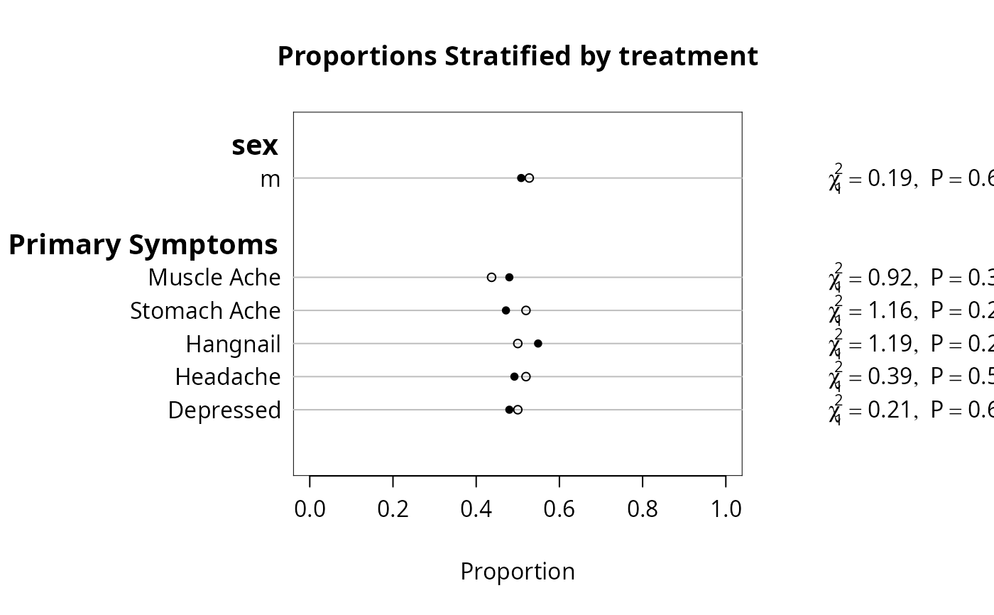
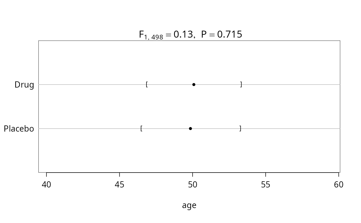
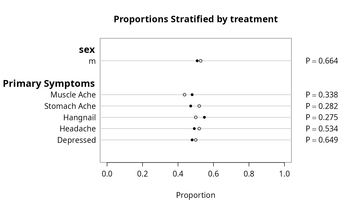
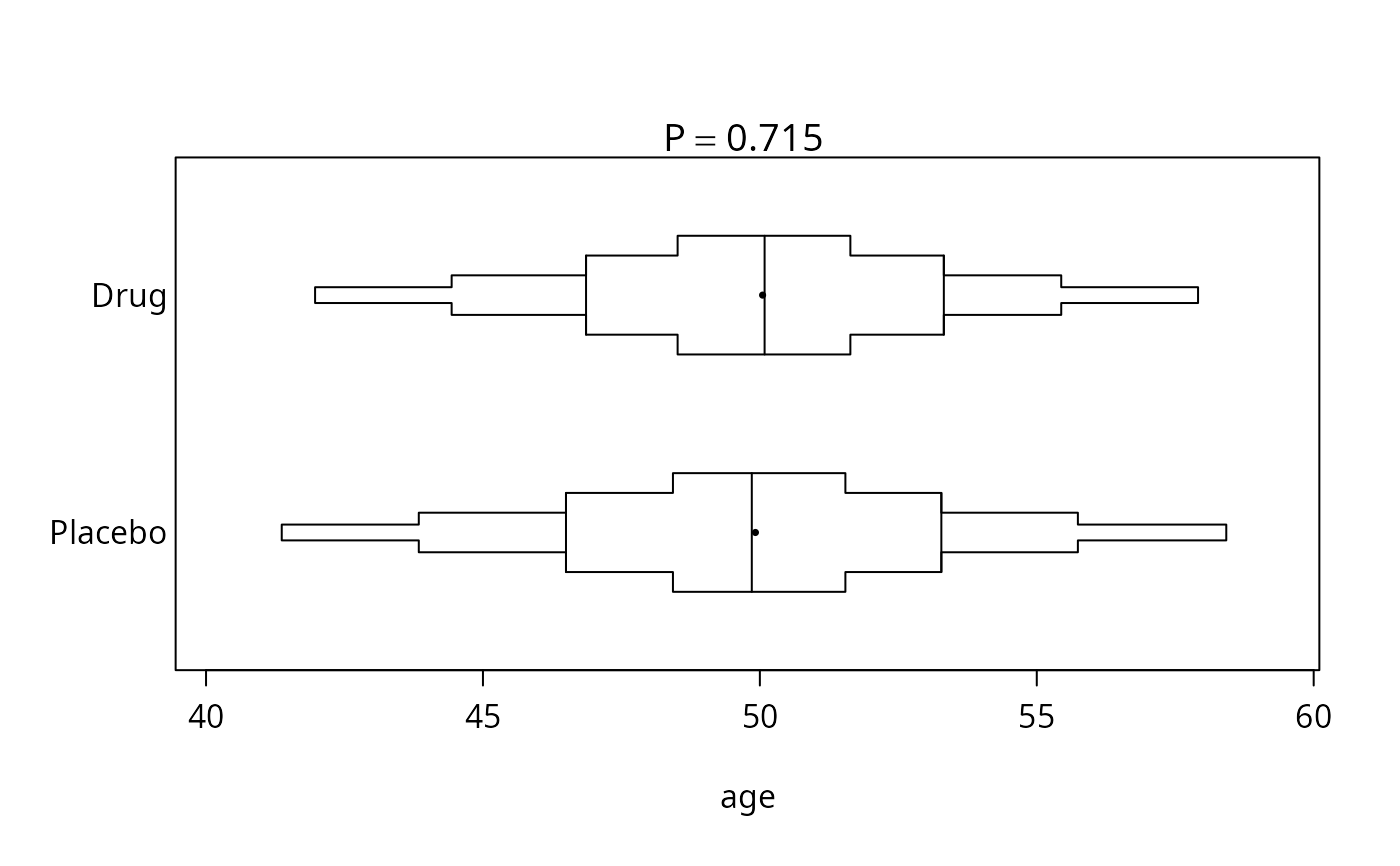
f <- summary(treatment ~ age + sex + Symptoms, method="reverse", test=TRUE)
f
#> 
#> 
#> Descriptive Statistics by treatment
#> 
#> +------------------------------+----------------------+----------------------+------------------------------+
#> |                              |Drug                  |Placebo               |  Test                        |
#> |                              |(N=246)               |(N=254)               |Statistic                     |
#> +------------------------------+----------------------+----------------------+------------------------------+
#> |age                           |        46.9/50.1/53.3|        46.5/49.9/53.3|   F=0.13 d.f.=1,498 P=0.715  |
#> +------------------------------+----------------------+----------------------+------------------------------+
#> |sex : m                       |          51%  (125)  |          53%  (134)  |Chi-square=0.19 d.f.=1 P=0.664|
#> +------------------------------+----------------------+----------------------+------------------------------+
#> |Primary Symptoms : Muscle Ache|          48%  (118)  |          44%  (111)  |Chi-square=0.92 d.f.=1 P=0.338|
#> +------------------------------+----------------------+----------------------+------------------------------+
#> |    Stomach Ache              |          47%  (116)  |          52%  (132)  |Chi-square=1.16 d.f.=1 P=0.282|
#> +------------------------------+----------------------+----------------------+------------------------------+
#> |    Hangnail                  |          55%  (135)  |          50%  (127)  |Chi-square=1.19 d.f.=1 P=0.275|
#> +------------------------------+----------------------+----------------------+------------------------------+
#> |    Headache                  |          49%  (121)  |          52%  (132)  |Chi-square=0.39 d.f.=1 P=0.534|
#> +------------------------------+----------------------+----------------------+------------------------------+
#> |    Depressed                 |          48%  (118)  |          50%  (127)  |Chi-square=0.21 d.f.=1 P=0.649|
#> +------------------------------+----------------------+----------------------+------------------------------+
# trio of numbers represent 25th, 50th, 75th percentile
print(f, long=TRUE)
#> 
#> 
#> Descriptive Statistics by treatment
#> 
#> +----------------+----------------------+----------------------+------------------------------+
#> |                |Drug                  |Placebo               |  Test                        |
#> |                |(N=246)               |(N=254)               |Statistic                     |
#> +----------------+----------------------+----------------------+------------------------------+
#> |age             |        46.9/50.1/53.3|        46.5/49.9/53.3|   F=0.13 d.f.=1,498 P=0.715  |
#> +----------------+----------------------+----------------------+------------------------------+
#> |sex             |                      |                      |Chi-square=0.19 d.f.=1 P=0.664|
#> +----------------+----------------------+----------------------+------------------------------+
#> |    m           |          51%  (125)  |          53%  (134)  |                              |
#> +----------------+----------------------+----------------------+------------------------------+
#> |Primary Symptoms|                      |                      |                              |
#> +----------------+----------------------+----------------------+------------------------------+
#> |    Muscle Ache |          48%  (118)  |          44%  (111)  |Chi-square=0.92 d.f.=1 P=0.338|
#> +----------------+----------------------+----------------------+------------------------------+
#> |    Stomach Ache|          47%  (116)  |          52%  (132)  |Chi-square=1.16 d.f.=1 P=0.282|
#> +----------------+----------------------+----------------------+------------------------------+
#> |    Hangnail    |          55%  (135)  |          50%  (127)  |Chi-square=1.19 d.f.=1 P=0.275|
#> +----------------+----------------------+----------------------+------------------------------+
#> |    Headache    |          49%  (121)  |          52%  (132)  |Chi-square=0.39 d.f.=1 P=0.534|
#> +----------------+----------------------+----------------------+------------------------------+
#> |    Depressed   |          48%  (118)  |          50%  (127)  |Chi-square=0.21 d.f.=1 P=0.649|
#> +----------------+----------------------+----------------------+------------------------------+
plot(f)


plot(f, conType='bp', prtest='P')


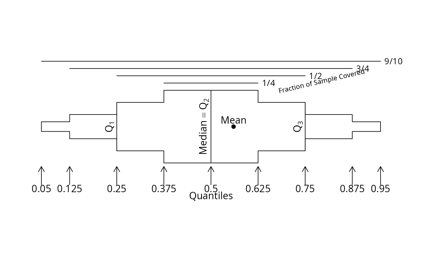
bpplt()    # annotated example showing layout of bp plot


#Compute predicted probability from a logistic regression model
#For different stratifications compute receiver operating
#characteristic curve areas (C-indexes)
predicted <- plogis(.4*(sex=="m")+.15*(age-50))
positive.diagnosis <- ifelse(runif(500)<=predicted, 1, 0)
roc <- function(z) {
   x <- z[,1];
   y <- z[,2];
   n <- length(x);
   if(n<2)return(c(ROC=NA));
   n1 <- sum(y==1);
   c(ROC= (mean(rank(x)[y==1])-(n1+1)/2)/(n-n1) );
 }
y <- cbind(predicted, positive.diagnosis)
options(digits=2)
summary(y ~ age + sex, fun=roc)
#> y      N= 500  
#> 
#> +-------+-----------+---+----+
#> |       |           |  N| ROC|
#> +-------+-----------+---+----+
#> |    age|[36.8,46.7)|125|0.60|
#> |       |[46.7,50.0)|125|0.55|
#> |       |[50.0,53.3)|125|0.62|
#> |       |[53.3,67.5]|125|0.62|
#> +-------+-----------+---+----+
#> |    sex|          f|241|0.72|
#> |       |          m|259|0.70|
#> +-------+-----------+---+----+
#> |Overall|           |500|0.72|
#> +-------+-----------+---+----+


options(digits=3)
summary(y ~ age + sex, fun=roc, method="cross")
#> 
#>  roc by age, sex 
#> 
#> +-+
#> |N|
#> |y|
#> +-+
#> +-----------+-----+-----+-----+
#> |    age    |  f  |  m  | ALL |
#> +-----------+-----+-----+-----+
#> |[36.8,46.7)|   65|   60|  125|
#> |           |0.526|0.626|0.598|
#> +-----------+-----+-----+-----+
#> |[46.7,50.0)|   65|   60|  125|
#> |           |0.588|0.467|0.554|
#> +-----------+-----+-----+-----+
#> |[50.0,53.3)|   53|   72|  125|
#> |           |0.567|0.652|0.622|
#> +-----------+-----+-----+-----+
#> |[53.3,67.5]|   58|   67|  125|
#> |           |0.646|0.622|0.618|
#> +-----------+-----+-----+-----+
#> |        ALL|  241|  259|  500|
#> |           |0.718|0.704|0.716|
#> +-----------+-----+-----+-----+

#Use stratify() to produce a table in which time intervals go down the
#page and going across 3 continuous variables are summarized using
#quartiles, and are stratified by two treatments

set.seed(1)
d <- expand.grid(visit=1:5, treat=c('A','B'), reps=1:100)
d$sysbp <- rnorm(100*5*2, 120, 10)
label(d$sysbp) <- 'Systolic BP'
d$diasbp <- rnorm(100*5*2, 80,  7)
d$diasbp[1] <- NA
d$age    <- rnorm(100*5*2, 50, 12)
g <- function(y) {
  N <- apply(y, 2, function(w) sum(!is.na(w)))
  h <- function(x) {
    qu <- quantile(x, c(.25,.5,.75), na.rm=TRUE)
    names(qu) <- c('Q1','Q2','Q3')
    c(N=sum(!is.na(x)), qu)
}
  w <- as.vector(apply(y, 2, h))
  names(w) <- as.vector( outer(c('N','Q1','Q2','Q3'), dimnames(y)[[2]],
                                function(x,y) paste(y,x)))
  w
}
#Use na.rm=FALSE to count NAs separately by column
s <- summary(cbind(age,sysbp,diasbp) ~ visit + stratify(treat),
             na.rm=FALSE, fun=g, data=d)
#The result is very wide.  Re-do, putting treatment vertically
x <- with(d, factor(paste('Visit', visit, treat)))
summary(cbind(age,sysbp,diasbp) ~ x, na.rm=FALSE, fun=g, data=d)
#> cbind(age, sysbp, diasbp)      N= 1000  
#> 
#> +-------+---------+----+-----+------+------+------+-------+--------+--------+--------+--------+---------+---------+---------+
#> |       |         |   N|age N|age Q1|age Q2|age Q3|sysbp N|sysbp Q1|sysbp Q2|sysbp Q3|diasbp N|diasbp Q1|diasbp Q2|diasbp Q3|
#> +-------+---------+----+-----+------+------+------+-------+--------+--------+--------+--------+---------+---------+---------+
#> |      x|Visit 1 A| 100|  100|  43.6|  49.8|  59.5|    100|     113|     118|     127|      99|     75.6|     79.3|     83.4|
#> |       |Visit 1 B| 100|  100|  42.1|  49.1|  56.5|    100|     111|     119|     127|     100|     75.8|     79.6|     84.1|
#> |       |Visit 2 A| 100|  100|  41.6|  48.1|  58.3|    100|     116|     122|     129|     100|     76.7|     79.9|     85.1|
#> |       |Visit 2 B| 100|  100|  43.3|  49.9|  58.0|    100|     113|     119|     127|     100|     73.4|     79.2|     86.0|
#> |       |Visit 3 A| 100|  100|  43.8|  51.0|  61.8|    100|     113|     120|     127|     100|     73.9|     78.9|     83.5|
#> |       |Visit 3 B| 100|  100|  42.3|  50.3|  58.9|    100|     115|     120|     127|     100|     75.8|     79.5|     85.3|
#> |       |Visit 4 A| 100|  100|  44.9|  50.1|  58.6|    100|     111|     117|     122|     100|     74.6|     81.4|     86.1|
#> |       |Visit 4 B| 100|  100|  38.6|  47.2|  56.2|    100|     113|     120|     126|     100|     74.3|     79.5|     84.7|
#> |       |Visit 5 A| 100|  100|  46.2|  52.1|  57.6|    100|     114|     120|     127|     100|     74.8|     80.6|     85.3|
#> |       |Visit 5 B| 100|  100|  39.2|  49.1|  59.5|    100|     115|     120|     127|     100|     76.9|     80.0|     84.5|
#> +-------+---------+----+-----+------+------+------+-------+--------+--------+--------+--------+---------+---------+---------+
#> |Overall|         |1000| 1000|  42.4|  49.9|  58.6|   1000|     113|     120|     127|     999|     75.1|     79.8|     85.2|
#> +-------+---------+----+-----+------+------+------+-------+--------+--------+--------+--------+---------+---------+---------+

#Compose LaTeX code directly
g <- function(y) {
  h <- function(x) {
    qu <- format(round(quantile(x, c(.25,.5,.75), na.rm=TRUE),1),nsmall=1)
    paste('{\\scriptsize(',sum(!is.na(x)),
          ')} \\hfill{\\scriptsize ', qu[1], '} \\textbf{', qu[2],
          '} {\\scriptsize ', qu[3],'}', sep='')
  }
  apply(y, 2, h)
}
s <- summary(cbind(age,sysbp,diasbp) ~ visit + stratify(treat),
             na.rm=FALSE, fun=g, data=d)
# latex(s, prn=FALSE)
## need option in latex to not print n
#Put treatment vertically
s <- summary(cbind(age,sysbp,diasbp) ~ x, fun=g, data=d, na.rm=FALSE)
# latex(s, prn=FALSE)

#Plot estimated mean life length (assuming an exponential distribution) 
#separately by levels of 4 other variables.  Repeat the analysis
#by levels of a stratification variable, drug.  Automatically break
#continuous variables into tertiles.
#We are using the default, method='response'
if (FALSE) { # \dontrun{
life.expect <- function(y) c(Years=sum(y[,1])/sum(y[,2]))
attach(pbc)
require(survival)
S <- Surv(follow.up.time, death)
s2 <- summary(S ~ age + albumin + ascites + edema + stratify(drug),
                         fun=life.expect, g=3)


#Note: You can summarize other response variables using the same 
#independent variables using e.g. update(s2, response~.), or you 
#can change the list of independent variables using e.g. 
#update(s2, response ~.- ascites) or update(s2, .~.-ascites)
#You can also print, typeset, or plot subsets of s2, e.g.
#plot(s2[c('age','albumin'),]) or plot(s2[1:2,])


s2    # invokes print.summary.formula.response


#Plot results as a separate dot chart for each of the 3 strata levels
par(mfrow=c(2,2))
plot(s2, cex.labels=.6, xlim=c(0,40), superposeStrata=FALSE)


#Typeset table, creating s2.tex
w <- latex(s2, cdec=1)
#Typeset table but just print LaTeX code
latex(s2, file="")    # useful for Sweave


#Take control of groups used for age.  Compute 3 quartiles for
#both cholesterol and bilirubin (excluding observations that are missing
#on EITHER ONE)


age.groups <- cut2(age, c(45,60))
g <- function(y) apply(y, 2, quantile, c(.25,.5,.75))
y <- cbind(Chol=chol,Bili=bili)
label(y) <- 'Cholesterol and Bilirubin'
#You can give new column names that are not legal S names
#by enclosing them in quotes, e.g. 'Chol (mg/dl)'=chol


s <- summary(y ~ age.groups + ascites, fun=g)


par(mfrow=c(1,2), oma=c(3,0,3,0))   # allow outer margins for overall
for(ivar in 1:2) {                  # title 
  isub <- (1:3)+(ivar-1)*3          # *3=number of quantiles/var.
  plot(s3, which=isub, main='', 
       xlab=c('Cholesterol','Bilirubin')[ivar],
       pch=c(91,16,93))            # [, closed circle, ]
  }
mtext(paste('Quartiles of', label(y)), adj=.5, outer=TRUE, cex=1.75)  
#Overall (outer) title


prlatex(latex(s3, trios=TRUE)) 
# trios -> collapse 3 quartiles


#Summarize only bilirubin, but do it with two statistics:
#the mean and the median.  Make separate tables for the two randomized
#groups and make plots for the active arm.


g <- function(y) c(Mean=mean(y), Median=median(y))


for(sub in c("D-penicillamine", "placebo")) {
  ss <- summary(bili ~ age.groups + ascites + chol, fun=g,
                subset=drug==sub)
  cat('\n',sub,'\n\n')
  print(ss)


  if(sub=='D-penicillamine') {
    par(mfrow=c(1,1))
    plot(s4, which=1:2, dotfont=c(1,-1), subtitles=FALSE, main='')
    #1=mean, 2=median     -1 font = open circle
    title(sub='Closed circle: mean;  Open circle: median', adj=0)
    title(sub=sub, adj=1)
  }


  w <- latex(ss, append=TRUE, fi='my.tex', 
             label=if(sub=='placebo') 's4b' else 's4a',
             caption=paste(label(bili),' {\\em (',sub,')}', sep=''))
  #Note symbolic labels for tables for two subsets: s4a, s4b
  prlatex(w)
}


#Now consider examples in 'reverse' format, where the lone dependent
#variable tells the summary function how to stratify all the 
#'independent' variables.  This is typically used to make tables 
#comparing baseline variables by treatment group, for example.


s5 <- summary(drug ~ bili + albumin + stage + protime + sex + 
                     age + spiders,
              method='reverse')
#To summarize all variables, use summary(drug ~., data=pbc)
#To summarize all variables with no stratification, use
#summary(~a+b+c) or summary(~.,data=\dots)


options(digits=1)
print(s5, npct='both')
#npct='both' : print both numerators and denominators
plot(s5, which='categorical')
Key(locator(1))  # draw legend at mouse click
par(oma=c(3,0,0,0))  # leave outer margin at bottom
plot(s5, which='continuous')
Key2()           # draw legend at lower left corner of plot
                 # oma= above makes this default key fit the page better


options(digits=3)
w <- latex(s5, npct='both', here=TRUE)     
# creates s5.tex


#Turn to a different dataset and do cross-classifications on possibly 
#more than one independent variable.  The summary function with 
#method='cross' produces a data frame containing the cross-
#classifications.  This data frame is suitable for multi-panel 
#trellis displays, although `summarize' works better for that.


attach(prostate)
size.quartile <- cut2(sz, g=4)
bone <- factor(bm,labels=c("no mets","bone mets"))


s7 <- summary(ap>1 ~ size.quartile + bone, method='cross')
#In this case, quartiles are the default so could have said sz + bone


options(digits=3)
print(s7, twoway=FALSE)
s7   # same as print(s7)
w <- latex(s7, here=TRUE)   # Make s7.tex


library(trellis,TRUE)
invisible(ps.options(reset=TRUE))
trellis.device(postscript, file='demo2.ps')


dotplot(S ~ size.quartile|bone, data=s7, #s7 is name of summary stats
                  xlab="Fraction ap>1", ylab="Quartile of Tumor Size")
#Can do this more quickly with summarize:
# s7 <- summarize(ap>1, llist(size=cut2(sz, g=4), bone), mean,
#                 stat.name='Proportion')
# dotplot(Proportion ~ size | bone, data=s7)


summary(age ~ stage, method='cross')
summary(age ~ stage, fun=quantile, method='cross')
summary(age ~ stage, fun=smean.sd, method='cross')
summary(age ~ stage, fun=smedian.hilow, method='cross')
summary(age ~ stage, fun=function(x) c(Mean=mean(x), Median=median(x)),
        method='cross')
#The next statements print real two-way tables
summary(cbind(age,ap) ~ stage + bone, 
        fun=function(y) apply(y, 2, quantile, c(.25,.75)),
        method='cross')
options(digits=2)
summary(log(ap) ~ sz + bone,
        fun=function(y) c(Mean=mean(y), quantile(y)),
        method='cross')


#Summarize an ordered categorical response by all of the needed
#cumulative proportions
summary(cumcategory(disease.severity) ~ age + sex)

} # }