Summarize Scalars or Matrices by Cross-Classification
summarize.Rdsummarize is a fast version of summary.formula(formula,
method="cross",overall=FALSE) for producing stratified summary statistics
and storing them in a data frame for plotting (especially with trellis
xyplot and dotplot and Hmisc xYplot). Unlike
aggregate, summarize accepts a matrix as its first
argument and a multi-valued FUN
argument and summarize also labels the variables in the new data
frame using their original names. Unlike methods based on
tapply, summarize stores the values of the stratification
variables using their original types, e.g., a numeric by variable
will remain a numeric variable in the collapsed data frame.
summarize also retains "label" attributes for variables.
summarize works especially well with the Hmisc xYplot
function for displaying multiple summaries of a single variable on each
panel, such as means and upper and lower confidence limits.
asNumericMatrix converts a data frame into a numeric matrix,
saving attributes to reverse the process by matrix2dataframe.
It saves attributes that are commonly preserved across row
subsetting (i.e., it does not save dim, dimnames, or
names attributes).
matrix2dataFrame converts a numeric matrix back into a data
frame if it was created by asNumericMatrix.
Usage
summarize(X, by, FUN, ...,
          stat.name=deparse(substitute(X)),
          type=c('variables','matrix'), subset=TRUE,
          keepcolnames=FALSE)

asNumericMatrix(x)

matrix2dataFrame(x, at=attr(x, 'origAttributes'), restoreAll=TRUE)
Arguments
- X
a vector or matrix capable of being operated on by the function specified as the
FUNargument- by
one or more stratification variables. If a single variable,
bymay be a vector, otherwise it should be a list. Using the Hmiscllistfunction instead oflistwill result in individual variable names being accessible tosummarize. For example, you can specifyllist(age.group,sex)orllist(Age=age.group,sex). The latter givesage.groupa new temporary name,Age.- FUN
a function of a single vector argument, used to create the statistical summaries for
summarize.FUNmay compute any number of statistics.- ...
extra arguments are passed to
FUN- stat.name
the name to use when creating the main summary variable. By default, the name of the
Xargument is used. Setstat.nametoNULLto suppress this name replacement.- type
Specify
type="matrix"to store the summary variables (if there are more than one) in a matrix.- subset
a logical vector or integer vector of subscripts used to specify the subset of data to use in the analysis. The default is to use all observations in the data frame.
- keepcolnames
by default when
type="matrix", the first column of the computed matrix is the name of the first argument tosummarize. Setkeepcolnames=TRUEto retain the name of the first column created byFUN- x
a data frame (for
asNumericMatrix) or a numeric matrix (formatrix2dataFrame).- at
List containing attributes of original data frame that survive subsetting. Defaults to attribute
"origAttributes"of the objectx, created by the call toasNumericMatrix- restoreAll
set to
FALSEto only restore attributeslabel,units, andlevelsinstead of all attributes
Value
For summarize, a data frame containing the by variables and the
statistical summaries (the first of which is named the same as the X
variable unless stat.name is given). If type="matrix", the
summaries are stored in a single variable in the data frame, and this
variable is a matrix.
asNumericMatrix returns a numeric matrix and stores an object
origAttributes as an attribute of the returned object, with original
attributes of component variables, the storage.mode.
matrix2dataFrame returns a data frame.
Author
Frank Harrell
Department of Biostatistics
Vanderbilt University
fh@fharrell.com
Examples
if (FALSE) { # \dontrun{
s <- summarize(ap>1, llist(size=cut2(sz, g=4), bone), mean,
stat.name='Proportion')
dotplot(Proportion ~ size | bone, data=s7)
} # }
set.seed(1)
temperature <- rnorm(300, 70, 10)
month <- sample(1:12, 300, TRUE)
year <- sample(2000:2001, 300, TRUE)
g <- function(x)c(Mean=mean(x,na.rm=TRUE),Median=median(x,na.rm=TRUE))
summarize(temperature, month, g)
#> month temperature Median
#> 1 1 68.6 69.4
#> 5 2 69.0 68.6
#> 6 3 68.9 68.1
#> 7 4 73.3 73.9
#> 8 5 69.5 71.8
#> 9 6 69.6 71.6
#> 10 7 72.4 69.4
#> 11 8 72.0 69.5
#> 12 9 69.5 68.3
#> 2 10 71.5 67.2
#> 3 11 70.7 70.7
#> 4 12 70.1 70.0
mApply(temperature, month, g)
#> Mean Median
#> 1 68.6 69.4
#> 2 69.0 68.6
#> 3 68.9 68.1
#> 4 73.3 73.9
#> 5 69.5 71.8
#> 6 69.6 71.6
#> 7 72.4 69.4
#> 8 72.0 69.5
#> 9 69.5 68.3
#> 10 71.5 67.2
#> 11 70.7 70.7
#> 12 70.1 70.0
mApply(temperature, month, mean, na.rm=TRUE)
#> 1 2 3 4 5 6 7 8 9 10 11 12
#> 68.6 69.0 68.9 73.3 69.5 69.6 72.4 72.0 69.5 71.5 70.7 70.1
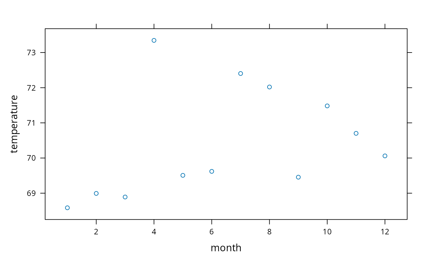
w <- summarize(temperature, month, mean, na.rm=TRUE)
library(lattice)
xyplot(temperature ~ month, data=w) # plot mean temperature by month
 w <- summarize(temperature, llist(year,month),
quantile, probs=c(.5,.25,.75), na.rm=TRUE, type='matrix')
xYplot(Cbind(temperature[,1],temperature[,-1]) ~ month | year, data=w)
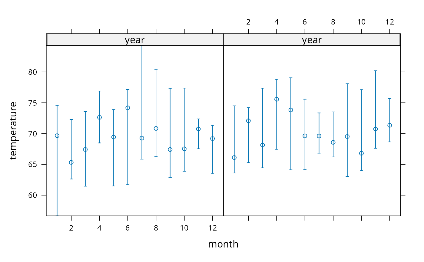
w <- summarize(temperature, llist(year,month),
quantile, probs=c(.5,.25,.75), na.rm=TRUE, type='matrix')
xYplot(Cbind(temperature[,1],temperature[,-1]) ~ month | year, data=w)
 mApply(temperature, llist(year,month),
quantile, probs=c(.5,.25,.75), na.rm=TRUE)
#> , , = 50%
#>
#> year
#> month 2000 2001
#> 1 69.7 66.1
#> 2 65.3 72.1
#> 3 67.4 68.1
#> 4 72.6 75.6
#> 5 69.4 73.8
#> 6 74.2 69.6
#> 7 69.3 69.6
#> 8 70.8 68.6
#> 9 67.4 69.5
#> 10 67.5 66.8
#> 11 70.8 70.7
#> 12 69.2 71.3
#>
#> , , = 25%
#>
#> year
#> month 2000 2001
#> 1 56.6 63.6
#> 2 62.6 65.3
#> 3 61.5 64.4
#> 4 68.5 67.4
#> 5 61.5 64.1
#> 6 61.7 64.2
#> 7 65.9 66.8
#> 8 66.2 66.2
#> 9 62.9 63.0
#> 10 63.9 64.0
#> 11 67.5 67.6
#> 12 63.6 68.6
#>
#> , , = 75%
#>
#> year
#> month 2000 2001
#> 1 74.6 74.5
#> 2 72.3 74.2
#> 3 73.6 77.4
#> 4 76.9 78.8
#> 5 73.9 79.1
#> 6 77.1 75.6
#> 7 84.3 73.4
#> 8 80.4 73.5
#> 9 77.4 78.1
#> 10 77.4 77.1
#> 11 72.4 80.2
#> 12 71.3 75.7
#>
# Compute the median and outer quartiles. The outer quartiles are
# displayed using "error bars"
set.seed(111)
dfr <- expand.grid(month=1:12, year=c(1997,1998), reps=1:100)
attach(dfr)
y <- abs(month-6.5) + 2*runif(length(month)) + year-1997
s <- summarize(y, llist(month,year), smedian.hilow, conf.int=.5)
s
#> month year y Lower Upper
#> 7 1 2000 9.03 8.92 9.35
#> 8 1 2001 10.73 9.97 11.15
#> 9 2 2000 8.89 8.69 9.17
#> 10 2 2001 9.48 9.13 9.83
#> 11 3 2000 7.15 6.81 8.02
#> 12 3 2001 8.76 8.30 9.39
#> 13 4 2000 6.29 5.77 7.02
#> 14 4 2001 7.21 6.93 7.83
#> 15 5 2000 5.30 5.06 5.75
#> 16 5 2001 6.58 5.71 6.79
#> 17 6 2000 4.65 4.42 4.81
#> 18 6 2001 5.56 5.04 5.99
#> 19 7 2000 5.02 4.28 5.19
#> 20 7 2001 5.02 4.64 5.33
#> 21 8 2000 5.66 5.54 5.80
#> 22 8 2001 6.53 6.21 7.13
#> 23 9 2000 6.73 6.04 7.16
#> 24 9 2001 7.96 7.31 8.37
#> 1 10 2000 7.67 7.12 8.19
#> 2 10 2001 8.60 7.96 8.82
#> 3 11 2000 9.00 8.65 9.27
#> 4 11 2001 9.30 8.84 9.73
#> 5 12 2000 9.03 8.65 9.60
#> 6 12 2001 10.69 10.27 11.11
mApply(y, llist(month,year), smedian.hilow, conf.int=.5)
#> , , = Median
#>
#> month
#> year 1 2 3 4 5 6 7 8 9 10 11 12
#> 2000 9.03 8.89 7.15 6.29 5.30 4.65 5.02 5.66 6.73 7.67 9.0 9.03
#> 2001 10.73 9.48 8.76 7.21 6.58 5.56 5.02 6.53 7.96 8.60 9.3 10.69
#>
#> , , = Lower
#>
#> month
#> year 1 2 3 4 5 6 7 8 9 10 11 12
#> 2000 8.92 8.69 6.81 5.77 5.06 4.42 4.28 5.54 6.04 7.12 8.65 8.65
#> 2001 9.97 9.13 8.30 6.93 5.71 5.04 4.64 6.21 7.31 7.96 8.84 10.27
#>
#> , , = Upper
#>
#> month
#> year 1 2 3 4 5 6 7 8 9 10 11 12
#> 2000 9.35 9.17 8.02 7.02 5.75 4.81 5.19 5.80 7.16 8.19 9.27 9.6
#> 2001 11.15 9.83 9.39 7.83 6.79 5.99 5.33 7.13 8.37 8.82 9.73 11.1
#>
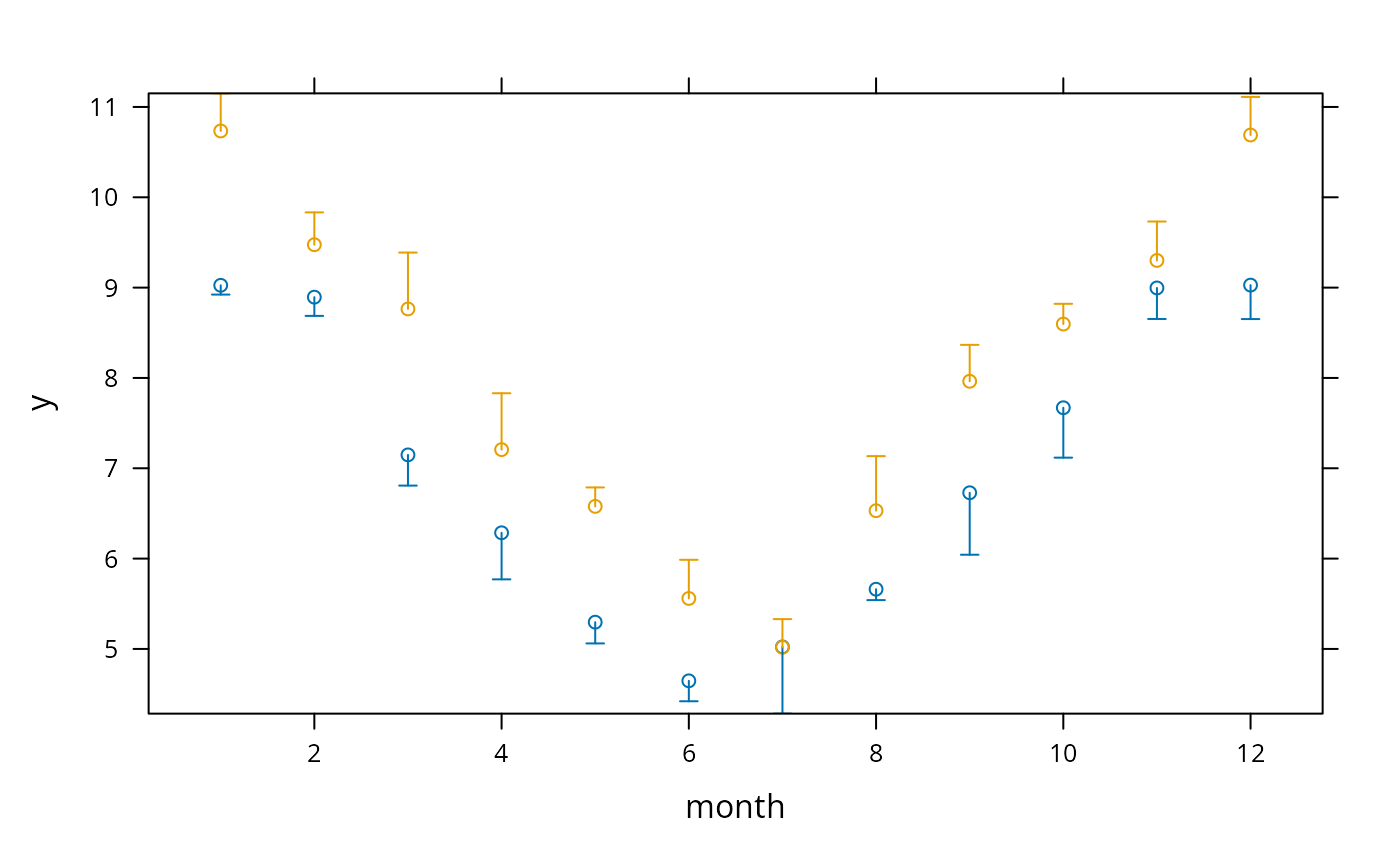
xYplot(Cbind(y,Lower,Upper) ~ month, groups=year, data=s,
keys='lines', method='alt')
mApply(temperature, llist(year,month),
quantile, probs=c(.5,.25,.75), na.rm=TRUE)
#> , , = 50%
#>
#> year
#> month 2000 2001
#> 1 69.7 66.1
#> 2 65.3 72.1
#> 3 67.4 68.1
#> 4 72.6 75.6
#> 5 69.4 73.8
#> 6 74.2 69.6
#> 7 69.3 69.6
#> 8 70.8 68.6
#> 9 67.4 69.5
#> 10 67.5 66.8
#> 11 70.8 70.7
#> 12 69.2 71.3
#>
#> , , = 25%
#>
#> year
#> month 2000 2001
#> 1 56.6 63.6
#> 2 62.6 65.3
#> 3 61.5 64.4
#> 4 68.5 67.4
#> 5 61.5 64.1
#> 6 61.7 64.2
#> 7 65.9 66.8
#> 8 66.2 66.2
#> 9 62.9 63.0
#> 10 63.9 64.0
#> 11 67.5 67.6
#> 12 63.6 68.6
#>
#> , , = 75%
#>
#> year
#> month 2000 2001
#> 1 74.6 74.5
#> 2 72.3 74.2
#> 3 73.6 77.4
#> 4 76.9 78.8
#> 5 73.9 79.1
#> 6 77.1 75.6
#> 7 84.3 73.4
#> 8 80.4 73.5
#> 9 77.4 78.1
#> 10 77.4 77.1
#> 11 72.4 80.2
#> 12 71.3 75.7
#>
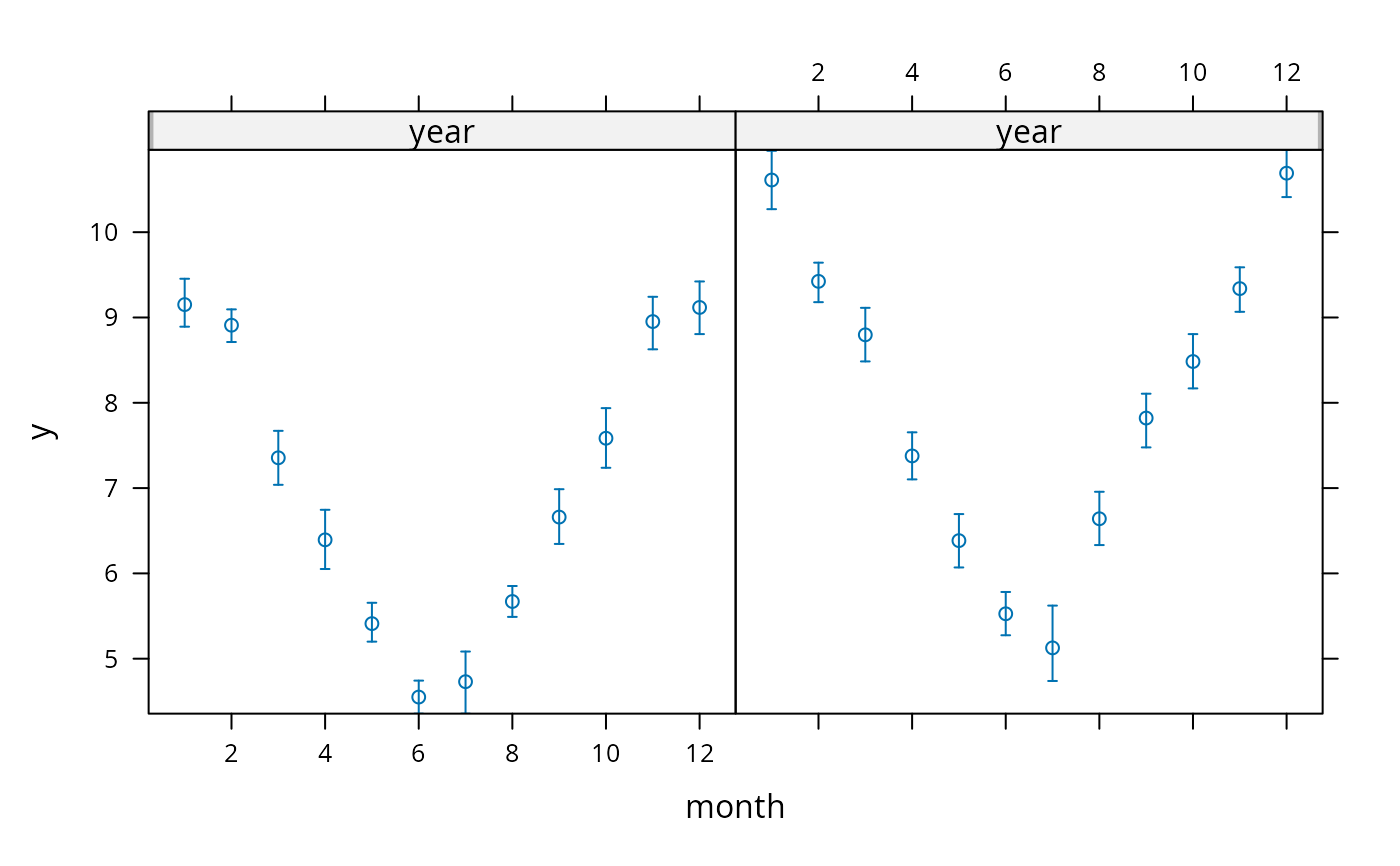
# Compute the median and outer quartiles. The outer quartiles are
# displayed using "error bars"
set.seed(111)
dfr <- expand.grid(month=1:12, year=c(1997,1998), reps=1:100)
attach(dfr)
y <- abs(month-6.5) + 2*runif(length(month)) + year-1997
s <- summarize(y, llist(month,year), smedian.hilow, conf.int=.5)
s
#> month year y Lower Upper
#> 7 1 2000 9.03 8.92 9.35
#> 8 1 2001 10.73 9.97 11.15
#> 9 2 2000 8.89 8.69 9.17
#> 10 2 2001 9.48 9.13 9.83
#> 11 3 2000 7.15 6.81 8.02
#> 12 3 2001 8.76 8.30 9.39
#> 13 4 2000 6.29 5.77 7.02
#> 14 4 2001 7.21 6.93 7.83
#> 15 5 2000 5.30 5.06 5.75
#> 16 5 2001 6.58 5.71 6.79
#> 17 6 2000 4.65 4.42 4.81
#> 18 6 2001 5.56 5.04 5.99
#> 19 7 2000 5.02 4.28 5.19
#> 20 7 2001 5.02 4.64 5.33
#> 21 8 2000 5.66 5.54 5.80
#> 22 8 2001 6.53 6.21 7.13
#> 23 9 2000 6.73 6.04 7.16
#> 24 9 2001 7.96 7.31 8.37
#> 1 10 2000 7.67 7.12 8.19
#> 2 10 2001 8.60 7.96 8.82
#> 3 11 2000 9.00 8.65 9.27
#> 4 11 2001 9.30 8.84 9.73
#> 5 12 2000 9.03 8.65 9.60
#> 6 12 2001 10.69 10.27 11.11
mApply(y, llist(month,year), smedian.hilow, conf.int=.5)
#> , , = Median
#>
#> month
#> year 1 2 3 4 5 6 7 8 9 10 11 12
#> 2000 9.03 8.89 7.15 6.29 5.30 4.65 5.02 5.66 6.73 7.67 9.0 9.03
#> 2001 10.73 9.48 8.76 7.21 6.58 5.56 5.02 6.53 7.96 8.60 9.3 10.69
#>
#> , , = Lower
#>
#> month
#> year 1 2 3 4 5 6 7 8 9 10 11 12
#> 2000 8.92 8.69 6.81 5.77 5.06 4.42 4.28 5.54 6.04 7.12 8.65 8.65
#> 2001 9.97 9.13 8.30 6.93 5.71 5.04 4.64 6.21 7.31 7.96 8.84 10.27
#>
#> , , = Upper
#>
#> month
#> year 1 2 3 4 5 6 7 8 9 10 11 12
#> 2000 9.35 9.17 8.02 7.02 5.75 4.81 5.19 5.80 7.16 8.19 9.27 9.6
#> 2001 11.15 9.83 9.39 7.83 6.79 5.99 5.33 7.13 8.37 8.82 9.73 11.1
#>
xYplot(Cbind(y,Lower,Upper) ~ month, groups=year, data=s,
keys='lines', method='alt')
 # Can also do:
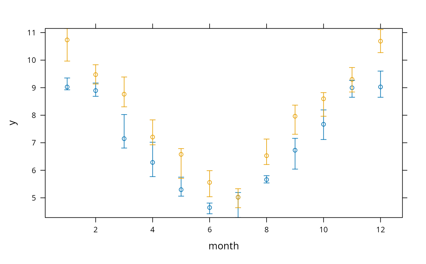
s <- summarize(y, llist(month,year), quantile, probs=c(.5,.25,.75),
stat.name=c('y','Q1','Q3'))
xYplot(Cbind(y, Q1, Q3) ~ month, groups=year, data=s, keys='lines')
# Can also do:
s <- summarize(y, llist(month,year), quantile, probs=c(.5,.25,.75),
stat.name=c('y','Q1','Q3'))
xYplot(Cbind(y, Q1, Q3) ~ month, groups=year, data=s, keys='lines')
 # To display means and bootstrapped nonparametric confidence intervals
# use for example:
s <- summarize(y, llist(month,year), smean.cl.boot)
xYplot(Cbind(y, Lower, Upper) ~ month | year, data=s)
# To display means and bootstrapped nonparametric confidence intervals
# use for example:
s <- summarize(y, llist(month,year), smean.cl.boot)
xYplot(Cbind(y, Lower, Upper) ~ month | year, data=s)
 # For each subject use the trapezoidal rule to compute the area under
# the (time,response) curve using the Hmisc trap.rule function
x <- cbind(time=c(1,2,4,7, 1,3,5,10),response=c(1,3,2,4, 1,3,2,4))
subject <- c(rep(1,4),rep(2,4))
trap.rule(x[1:4,1],x[1:4,2])
#> [1] 16
summarize(x, subject, function(y) trap.rule(y[,1],y[,2]))
#> subject x
#> 1 1 16
#> 2 2 24
if (FALSE) { # \dontrun{
# Another approach would be to properly re-shape the mm array below
# This assumes no missing cells. There are many other approaches.
# mApply will do this well while allowing for missing cells.
m <- tapply(y, list(year,month), quantile, probs=c(.25,.5,.75))
mm <- array(unlist(m), dim=c(3,2,12),
dimnames=list(c('lower','median','upper'),c('1997','1998'),
as.character(1:12)))
# aggregate will help but it only allows you to compute one quantile
# at a time; see also the Hmisc mApply function
dframe <- aggregate(y, list(Year=year,Month=month), quantile, probs=.5)
# Compute expected life length by race assuming an exponential
# distribution - can also use summarize
g <- function(y) { # computations for one race group
futime <- y[,1]; event <- y[,2]
sum(futime)/sum(event) # assume event=1 for death, 0=alive
}
mApply(cbind(followup.time, death), race, g)
# To run mApply on a data frame:
xn <- asNumericMatrix(x)
m <- mApply(xn, race, h)
# Here assume h is a function that returns a matrix similar to x
matrix2dataFrame(m)
# Get stratified weighted means
g <- function(y) wtd.mean(y[,1],y[,2])
summarize(cbind(y, wts), llist(sex,race), g, stat.name='y')
mApply(cbind(y,wts), llist(sex,race), g)
# Compare speed of mApply vs. by for computing
d <- data.frame(sex=sample(c('female','male'),100000,TRUE),
country=sample(letters,100000,TRUE),
y1=runif(100000), y2=runif(100000))
g <- function(x) {
y <- c(median(x[,'y1']-x[,'y2']),
med.sum =median(x[,'y1']+x[,'y2']))
names(y) <- c('med.diff','med.sum')
y
}
system.time(by(d, llist(sex=d$sex,country=d$country), g))
system.time({
x <- asNumericMatrix(d)
a <- subsAttr(d)
m <- mApply(x, llist(sex=d$sex,country=d$country), g)
})
system.time({
x <- asNumericMatrix(d)
summarize(x, llist(sex=d$sex, country=d$country), g)
})
# An example where each subject has one record per diagnosis but sex of
# subject is duplicated for all the rows a subject has. Get the cross-
# classified frequencies of diagnosis (dx) by sex and plot the results
# with a dot plot
count <- rep(1,length(dx))
d <- summarize(count, llist(dx,sex), sum)
Dotplot(dx ~ count | sex, data=d)
} # }
d <- list(x=1:10, a=factor(rep(c('a','b'), 5)),
b=structure(letters[1:10], label='label for b'),
d=c(rep(TRUE,9), FALSE), f=pi*(1 : 10))
x <- asNumericMatrix(d)
attr(x, 'origAttributes')
#> $x
#> $x$.type.
#> [1] "integer"
#>
#>
#> $a
#> $a$levels
#> [1] "a" "b"
#>
#> $a$class
#> [1] "factor"
#>
#> $a$.type.
#> [1] "integer"
#>
#>
#> $b
#> $b$label
#> [1] "label for b"
#>
#> $b$levels
#> [1] "a" "b" "c" "d" "e" "f" "g" "h" "i" "j"
#>
#> $b$class
#> [1] "factor"
#>
#> $b$.type.
#> [1] "character"
#>
#>
#> $d
#> $d$.type.
#> [1] "logical"
#>
#>
#> $f
#> $f$.type.
#> [1] "double"
#>
#>
matrix2dataFrame(x)
#> x a b d f
#> 1 1 a a TRUE 3.14
#> 2 2 b b TRUE 6.28
#> 3 3 a c TRUE 9.42
#> 4 4 b d TRUE 12.57
#> 5 5 a e TRUE 15.71
#> 6 6 b f TRUE 18.85
#> 7 7 a g TRUE 21.99
#> 8 8 b h TRUE 25.13
#> 9 9 a i TRUE 28.27
#> 10 10 b j FALSE 31.42
detach('dfr')
# Run summarize on a matrix to get column means
x <- c(1:19,NA)
y <- 101:120
z <- cbind(x, y)
g <- c(rep(1, 10), rep(2, 10))
summarize(z, g, colMeans, na.rm=TRUE, stat.name='x')
#> g x y
#> 1 1 5.5 106
#> 2 2 15.0 116
# Also works on an all numeric data frame
summarize(as.data.frame(z), g, colMeans, na.rm=TRUE, stat.name='x')
#> g x y
#> 1 1 5.5 106
#> 2 2 15.0 116
# For each subject use the trapezoidal rule to compute the area under
# the (time,response) curve using the Hmisc trap.rule function
x <- cbind(time=c(1,2,4,7, 1,3,5,10),response=c(1,3,2,4, 1,3,2,4))
subject <- c(rep(1,4),rep(2,4))
trap.rule(x[1:4,1],x[1:4,2])
#> [1] 16
summarize(x, subject, function(y) trap.rule(y[,1],y[,2]))
#> subject x
#> 1 1 16
#> 2 2 24
if (FALSE) { # \dontrun{
# Another approach would be to properly re-shape the mm array below
# This assumes no missing cells. There are many other approaches.
# mApply will do this well while allowing for missing cells.
m <- tapply(y, list(year,month), quantile, probs=c(.25,.5,.75))
mm <- array(unlist(m), dim=c(3,2,12),
dimnames=list(c('lower','median','upper'),c('1997','1998'),
as.character(1:12)))
# aggregate will help but it only allows you to compute one quantile
# at a time; see also the Hmisc mApply function
dframe <- aggregate(y, list(Year=year,Month=month), quantile, probs=.5)
# Compute expected life length by race assuming an exponential
# distribution - can also use summarize
g <- function(y) { # computations for one race group
futime <- y[,1]; event <- y[,2]
sum(futime)/sum(event) # assume event=1 for death, 0=alive
}
mApply(cbind(followup.time, death), race, g)
# To run mApply on a data frame:
xn <- asNumericMatrix(x)
m <- mApply(xn, race, h)
# Here assume h is a function that returns a matrix similar to x
matrix2dataFrame(m)
# Get stratified weighted means
g <- function(y) wtd.mean(y[,1],y[,2])
summarize(cbind(y, wts), llist(sex,race), g, stat.name='y')
mApply(cbind(y,wts), llist(sex,race), g)
# Compare speed of mApply vs. by for computing
d <- data.frame(sex=sample(c('female','male'),100000,TRUE),
country=sample(letters,100000,TRUE),
y1=runif(100000), y2=runif(100000))
g <- function(x) {
y <- c(median(x[,'y1']-x[,'y2']),
med.sum =median(x[,'y1']+x[,'y2']))
names(y) <- c('med.diff','med.sum')
y
}
system.time(by(d, llist(sex=d$sex,country=d$country), g))
system.time({
x <- asNumericMatrix(d)
a <- subsAttr(d)
m <- mApply(x, llist(sex=d$sex,country=d$country), g)
})
system.time({
x <- asNumericMatrix(d)
summarize(x, llist(sex=d$sex, country=d$country), g)
})
# An example where each subject has one record per diagnosis but sex of
# subject is duplicated for all the rows a subject has. Get the cross-
# classified frequencies of diagnosis (dx) by sex and plot the results
# with a dot plot
count <- rep(1,length(dx))
d <- summarize(count, llist(dx,sex), sum)
Dotplot(dx ~ count | sex, data=d)
} # }
d <- list(x=1:10, a=factor(rep(c('a','b'), 5)),
b=structure(letters[1:10], label='label for b'),
d=c(rep(TRUE,9), FALSE), f=pi*(1 : 10))
x <- asNumericMatrix(d)
attr(x, 'origAttributes')
#> $x
#> $x$.type.
#> [1] "integer"
#>
#>
#> $a
#> $a$levels
#> [1] "a" "b"
#>
#> $a$class
#> [1] "factor"
#>
#> $a$.type.
#> [1] "integer"
#>
#>
#> $b
#> $b$label
#> [1] "label for b"
#>
#> $b$levels
#> [1] "a" "b" "c" "d" "e" "f" "g" "h" "i" "j"
#>
#> $b$class
#> [1] "factor"
#>
#> $b$.type.
#> [1] "character"
#>
#>
#> $d
#> $d$.type.
#> [1] "logical"
#>
#>
#> $f
#> $f$.type.
#> [1] "double"
#>
#>
matrix2dataFrame(x)
#> x a b d f
#> 1 1 a a TRUE 3.14
#> 2 2 b b TRUE 6.28
#> 3 3 a c TRUE 9.42
#> 4 4 b d TRUE 12.57
#> 5 5 a e TRUE 15.71
#> 6 6 b f TRUE 18.85
#> 7 7 a g TRUE 21.99
#> 8 8 b h TRUE 25.13
#> 9 9 a i TRUE 28.27
#> 10 10 b j FALSE 31.42
detach('dfr')
# Run summarize on a matrix to get column means
x <- c(1:19,NA)
y <- 101:120
z <- cbind(x, y)
g <- c(rep(1, 10), rep(2, 10))
summarize(z, g, colMeans, na.rm=TRUE, stat.name='x')
#> g x y
#> 1 1 5.5 106
#> 2 2 15.0 116
# Also works on an all numeric data frame
summarize(as.data.frame(z), g, colMeans, na.rm=TRUE, stat.name='x')
#> g x y
#> 1 1 5.5 106
#> 2 2 15.0 116