Summarize Mixed Data Types vs. Groups

summaryM summarizes the variables listed in an S formula, computing descriptive statistics and optionally statistical tests for group differences. This function is typically used when there are multiple left-hand-side variables that are independently against by groups marked by a single right-hand-side variable. The summary statistics may be passed to print methods, plot methods for making annotated dot charts and extended box plots, and latex methods for typesetting tables using LaTeX. The html method uses htmlTable::htmlTable to typeset the table in html, by passing information to the latex method with html=TRUE. This is for use with Quarto/RMarkdown. The print methods use the print.char.matrix function to print boxed tables when options(prType=) has not been given or when prType='plain'. For plain tables, print calls the internal function printsummaryM. When prType='latex' the latex method is invoked, and when prType='html' html is rendered. In Quarto/RMarkdown, proper rendering will result even if results='asis' does not appear in the chunk header. When rendering in html at the console due to having options(prType='html') the table will be rendered in a viewer.

The plot method creates plotly graphics if options(grType='plotly'), otherwise base graphics are used. plotly graphics provide extra information such as which quantile is being displayed when hovering the mouse. Test statistics are displayed by hovering over the mean.

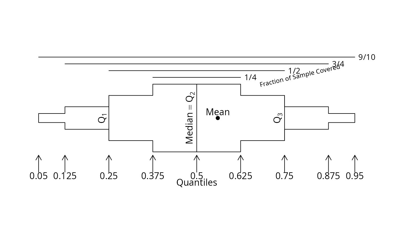
Continuous variables are described by three quantiles (quartiles by default) when printing, or by the following quantiles when plotting expended box plots using the bpplt function: 0.05, 0.125, 0.25, 0.375, 0.5, 0.625, 0.75, 0.875, 0.95. The box plots are scaled to the 0.025 and 0.975 quantiles of each continuous left-hand-side variable. Categorical variables are described by counts and percentages.

The left hand side of formula may contain mChoice ("multiple choice") variables. When test=TRUE each choice is tested separately as a binary categorical response.

The plot method for method="reverse" creates a temporary function Key as is done by the xYplot and Ecdf.formula functions. After plot runs, you can type Key() to put a legend in a default location, or e.g. Key(locator(1)) to draw a legend where you click the left mouse button. This key is for categorical variables, so to have the opportunity to put the key on the graph you will probably want to use the command plot(object, which="categorical"). A second function Key2 is created if continuous variables are being plotted. It is used the same as Key. If the which argument is not specified to plot, two pages of plots will be produced. If you don't define par(mfrow=) yourself, plot.summaryM will try to lay out a multi-panel graph to best fit all the individual charts for continuous variables.

Usage

summaryM(formula, groups=NULL, data=NULL, subset, na.action=na.retain,
         overall=FALSE, continuous=10, na.include=FALSE,
         quant=c(0.025, 0.05, 0.125, 0.25, 0.375, 0.5, 0.625,
                 0.75, 0.875, 0.95, 0.975),
         nmin=100, test=FALSE,
         conTest=conTestkw, catTest=catTestchisq,
         ordTest=ordTestpo)

# S3 method for class 'summaryM'
print(...)

printsummaryM(x, digits, prn = any(n != N),
      what=c('proportion', '%'), pctdig = if(what == '%') 0 else 2,
      npct = c('numerator', 'both', 'denominator', 'none'),
      exclude1 = TRUE, vnames = c('labels', 'names'), prUnits = TRUE,
      sep = '/', abbreviate.dimnames = FALSE,
      prefix.width = max(nchar(lab)), min.colwidth, formatArgs=NULL, round=NULL,
      prtest = c('P','stat','df','name'), prmsd = FALSE, long = FALSE,
      pdig = 3, eps = 0.001, prob = c(0.25, 0.5, 0.75), prN = FALSE, ...)

# S3 method for class 'summaryM'
plot(x, vnames = c('labels', 'names'),
     which = c('both', 'categorical', 'continuous'), vars=NULL,
     xlim = c(0,1),
     xlab = 'Proportion',
     pch = c(16, 1, 2, 17, 15, 3, 4, 5, 0), exclude1 = TRUE,
     main, ncols=2,
     prtest = c('P', 'stat', 'df', 'name'), pdig = 3, eps = 0.001,
     conType = c('bp', 'dot', 'raw'), cex.means = 0.5, cex=par('cex'),
     height='auto', width=700, ...)

# S3 method for class 'summaryM'
latex(object, title =
      first.word(deparse(substitute(object))),
      file=paste(title, 'tex', sep='.'), append=FALSE, digits, 
      prn = any(n != N), what=c('proportion', '%'),
      pctdig = if(what == '%') 0 else 2,
      npct = c('numerator', 'both', 'denominator', 'slash', 'none'),
      npct.size = if(html) mspecs$html$smaller else 'scriptsize',
      Nsize = if(html) mspecs$html$smaller else 'scriptsize',
      exclude1 = TRUE,
      vnames=c("labels", "names"), prUnits = TRUE, middle.bold = FALSE,
      outer.size = if(html) mspecs$html$smaller else "scriptsize",
      caption, rowlabel = "", rowsep=html,
      insert.bottom = TRUE, dcolumn = FALSE, formatArgs=NULL, round=NULL,
      prtest = c('P', 'stat', 'df', 'name'), prmsd = FALSE,
      msdsize = if(html) function(x) x else NULL, brmsd=FALSE,
      long = FALSE, pdig = 3, eps = 0.001,
      auxCol = NULL, table.env=TRUE, tabenv1=FALSE, prob=c(0.25, 0.5, 0.75),
      prN=FALSE, legend.bottom=FALSE, html=FALSE,
      mspecs=markupSpecs, ...)

# S3 method for class 'summaryM'
html(object, ...)

Arguments

formula

An S formula with additive effects. There may be several variables on the right hand side separated by "+", or the numeral 1, indicating that there is no grouping variable so that only margin summaries are produced. The right hand side variable, if present, must be a discrete variable producing a limited number of groups. On the left hand side there may be any number of variables, separated by "+", and these may be of mixed types. These variables are analyzed separately by the grouping variable.

groups

if there is more than one right-hand variable, specify groups as a character string containing the name of the variable used to produce columns of the table. The remaining right hand variables are combined to produce levels that cause separate tables or plots to be produced.

x

an object created by summaryM. For conTestkw a numeric vector, and for ordTestpo, a numeric or factor variable that can be considered ordered

data

name or number of a data frame. Default is the current frame.

subset

a logical vector or integer vector of subscripts used to specify the subset of data to use in the analysis. The default is to use all observations in the data frame.

na.action

function for handling missing data in the input data. The default is a function defined here called na.retain, which keeps all observations for processing, with missing variables or not.

overall

Setting overall=TRUE makes a new column with overall statistics for the whole sample. If test=TRUE these marginal statistics are ignored in doing statistical tests.

continuous

specifies the threshold for when a variable is considered to be continuous (when there are at least continuous unique values). factor variables are always considered to be categorical no matter how many levels they have.

na.include

Set na.include=TRUE to keep missing values of categorical variables from being excluded from the table.

nmin

For categories of the response variable in which there are less than or equal to nmin non-missing observations, the raw data are retained for later plotting in place of box plots.

test

Set to TRUE to compute test statistics using tests specified in conTest and catTest.

conTest

a function of two arguments (grouping variable and a continuous variable) that returns a list with components P (the computed P-value), stat (the test statistic, either chi-square or F), df (degrees of freedom), testname (test name), namefun ("chisq", "fstat"), statname (statistic name), an optional component latexstat (LaTeX representation of statname), an optional component plotmathstat (for R - the plotmath representation of statname, as a character string), and an optional component note that contains a character string note about the test (e.g., "test not done because n < 5"). conTest is applied to continuous variables on the right-hand-side of the formula when method="reverse". The default uses the spearman2 function to run the Wilcoxon or Kruskal-Wallis test using the F distribution.

catTest

a function of a frequency table (an integer matrix) that returns a list with the same components as created by conTest. By default, the Pearson chi-square test is done, without continuity correction (the continuity correction would make the test conservative like the Fisher exact test).

ordTest

a function of a frequency table (an integer matrix) that returns a list with the same components as created by conTest. By default, the Proportional odds likelihood ratio test is done.

...

For Key and Key2 these arguments are passed to key, text, or mtitle. For print methods these are optional arguments to print.char.matrix. For latex methods these are passed to latex.default. For html the arguments are passed the latex.summaryM, and the arguments may not include file. For print the arguments are passed to printsummaryM or latex.summaryM depending on options(prType=).

object

an object created by summaryM

quant

vector of quantiles to use for summarizing continuous variables. These must be numbers between 0 and 1 inclusive and must include the numbers 0.5, 0.25, and 0.75 which are used for printing and for plotting quantile intervals. The outer quantiles are used for scaling the x-axes for such plots. Specify outer quantiles as 0 and 1 to scale the x-axes using the whole observed data ranges instead of the default (a 0.95 quantile interval). Box-percentile plots are drawn using all but the outer quantiles.

prob

vector of quantiles to use for summarizing continuous variables. These must be numbers between 0 and 1 inclusive and have previously been included in the quant argument of summaryM. The vector must be of length three. By default it contains 0.25, 0.5, and 0.75.

Warning: specifying 0 and 1 as two of the quantiles will result in computing the minimum and maximum of the variable. As for many random variables the minimum will continue to become smaller as the sample size grows, and the maximum will continue to get larger. Thus the min and max are not recommended as summary statistics.

vnames

By default, tables and plots are usually labeled with variable labels (see the label and sas.get functions). To use the shorter variable names, specify vnames="name".

pch

vector of plotting characters to represent different groups, in order of group levels.

abbreviate.dimnames

see print.char.matrix

prefix.width

see print.char.matrix

min.colwidth

minimum column width to use for boxes printed with print.char.matrix. The default is the maximum of the minimum column label length and the minimum length of entries in the data cells.

formatArgs

a list containing other arguments to pass to format.default such as scientific, e.g., formatArgs=list(scientific=c(-5,5)). For print.summary.formula.reverse and format.summary.formula.reverse, formatArgs applies only to statistics computed on continuous variables, not to percents, numerators, and denominators. The round argument may be preferred.

digits

number of significant digits to print. Default is to use the current value of the digits system option.

what

specifies whether proportions or percentages are to be printed or LaTeX'd

pctdig

number of digits to the right of the decimal place for printing percentages or proportions. The default is zero if what='%', so percents will be rounded to the nearest percent. The default is 2 for proportions.

prn

set to TRUE to print the number of non-missing observations on the current (row) variable. The default is to print these only if any of the counts of non-missing values differs from the total number of non-missing values of the left-hand-side variable.

prN

set to TRUE to print the number of non-missing observations on rows that contain continuous variables.

npct

specifies which counts are to be printed to the right of percentages. The default is to print the frequency (numerator of the percent) in parentheses. You can specify "both" to print both numerator and denominator as a fraction, "denominator", "slash" to typeset horizontally using a forward slash, or "none".

npct.size

the size for typesetting npct information which appears after percents. The default is "scriptsize".

Nsize

When a second row of column headings is added showing sample sizes, Nsize specifies the LaTeX size for these subheadings. Default is "scriptsize".

exclude1

By default, summaryM objects will be printed, plotted, or typeset by removing redundant entries from percentage tables for categorical variables. For example, if you print the percent of females, you don't need to print the percent of males. To override this, set exclude1=FALSE.

prUnits

set to FALSE to suppress printing or latexing units attributes of variables, when method='reverse' or 'response'

sep

character to use to separate quantiles when printing tables

prtest

a vector of test statistic components to print if test=TRUE was in effect when summaryM was called. Defaults to printing all components. Specify prtest=FALSE or prtest="none" to not print any tests. This applies to print, latex, and plot methods.

round

Specify round to round the quantiles and optional mean and standard deviation to round digits after the decimal point. Set round='auto' to try an automatic choice.

prmsd

set to TRUE to print mean and SD after the three quantiles, for continuous variables

msdsize

defaults to NULL to use the current font size for the mean and standard deviation if prmsd is TRUE. Set to a character string or function to specify an alternate LaTeX font size.

brmsd

set to TRUE to put the mean and standard deviation on a separate line, for html

long

set to TRUE to print the results for the first category on its own line, not on the same line with the variable label

pdig

number of digits to the right of the decimal place for printing P-values. Default is 3. This is passed to format.pval.

eps

P-values less than eps will be printed as < eps. See format.pval.

auxCol

an optional auxiliary column of information, right justified, to add in front of statistics typeset by latex.summaryM. This argument is a list with a single element that has a name specifying the column heading. If this name includes a newline character, the portions of the string before and after the newline form respectively the main heading and the subheading (typically set in smaller font), respectively. See the extracolheads argument to latex.default. auxCol is filled with blanks when a variable being summarized takes up more than one row in the output. This happens with categorical variables.

table.env

set to FALSE to use tabular environment with no caption

tabenv1

set to TRUE in the case of stratification when you want only the first stratum's table to be in a table environment. This is useful when using hyperref.

which

Specifies whether to plot results for categorical variables, continuous variables, or both (the default).

vars

Subscripts (indexes) of variables to plot for plotly graphics. Default is to plot all variables of each type (categorical or continuous).

conType

For drawing plots for continuous variables, extended box plots (box-percentile-type plots) are drawn by default, using all quantiles in quant except for the outermost ones which are using for scaling the overall plot based on the non-stratified marginal distribution of the current response variable. Specify conType='dot' to draw dot plots showing the three quartiles instead. For extended box plots, means are drawn with a solid dot and vertical reference lines are placed at the three quartiles. Specify conType='raw' to make a strip chart showing the raw data. This can only be used if the sample size for each right-hand-side group is less than or equal to nmin.

cex.means

character size for means in box-percentile plots; default is .5

cex

character size for other plotted items

height,width

dimensions in pixels for the plotly subplot object containing all the extended box plots. If height="auto", plot.summaryM will set height based on the number of continuous variables and ncols or for dot charts it will use Hmisc::plotlyHeightDotchart. At present height is ignored for extended box plots due to vertical spacing problem with plotly graphics.

xlim

vector of length two specifying x-axis limits. This is only used for plotting categorical variables. Limits for continuous variables are determined by the outer quantiles specified in quant.

xlab

x-axis label

main

a main title. This applies only to the plot for categorical variables.

ncols

number of columns for plotly graphics for extended box plots. Defaults to 2. Recommendation is for 1-2.

caption

character string containing LaTeX table captions.

title

name of resulting LaTeX file omitting the .tex suffix. Default is the name of the summary object. If caption is specied, title is also used for the table's symbolic reference label.

file

name of file to write LaTeX code to. Specifying file="" will cause LaTeX code to just be printed to standard output rather than be stored in a permanent file.

append

specify TRUE to add code to an existing file

rowlabel

see latex.default (under the help file latex)

rowsep

if html is TRUE, instructs the function to use a horizontal line to separate variables from one another. Recommended if brmsd is TRUE. Ignored for LaTeX.

middle.bold

set to TRUE to have LaTeX use bold face for the middle quantile

outer.size

the font size for outer quantiles

insert.bottom

set to FALSE to suppress inclusion of definitions placed at the bottom of LaTeX tables. You can also specify a character string containing other text that overrides the automatic text. At present such text always appears in the main caption for LaTeX.

legend.bottom

set to TRUE to separate the table caption and legend. This will place table legends at the bottom of LaTeX tables.

html

set to TRUE to typeset with html

mspecs

list defining markup syntax for various languages, defaults to Hmisc markupSpecs which the user can use as a starting point for editing

dcolumn

see latex

Value

a list. plot.summaryM returns the number of pages of plots that were made if using base graphics, or plotly objects created by plotly::subplot otherwise. If both categorical and continuous variables were plotted, the returned object is a list with two named elements Categorical and Continuous each containing plotly objects. Otherwise a plotly object is returned. The latex method returns attributes legend and nstrata.

Side Effects

plot.summaryM creates a function Key and Key2 in frame 0 that will draw legends, if base graphics are being used.

Author

Frank Harrell
Department of Biostatistics
Vanderbilt University
fh@fharrell.com

References

Harrell FE (2004): Statistical tables and plots using S and LaTeX. Document available from https://hbiostat.org/R/Hmisc/summary.pdf.

See also

mChoice, label, dotchart3, print.char.matrix, update, formula, format.default, latex, latexTranslate, bpplt, tabulr, bpplotM, summaryP

Examples

options(digits=3)
set.seed(173)
sex <- factor(sample(c("m","f"), 500, rep=TRUE))
country <- factor(sample(c('US', 'Canada'), 500, rep=TRUE))
age <- rnorm(500, 50, 5)
sbp <- rnorm(500, 120, 12)
label(sbp) <- 'Systolic BP'
units(sbp) <- 'mmHg'
treatment <- factor(sample(c("Drug","Placebo"), 500, rep=TRUE))
treatment[1]
#> [1] Placebo
#> Levels: Drug Placebo
sbp[1] <- NA

# Generate a 3-choice variable; each of 3 variables has 5 possible levels
symp <- c('Headache','Stomach Ache','Hangnail',
          'Muscle Ache','Depressed')
symptom1 <- sample(symp, 500,TRUE)
symptom2 <- sample(symp, 500,TRUE)
symptom3 <- sample(symp, 500,TRUE)
Symptoms <- mChoice(symptom1, symptom2, symptom3, label='Primary Symptoms')
table(as.character(Symptoms))
#> 
#>                          Depressed              Depressed;Muscle Ache 
#>                                  5                                 24 
#>                           Hangnail                 Hangnail;Depressed 
#>                                  3                                 24 
#>     Hangnail;Depressed;Muscle Ache               Hangnail;Muscle Ache 
#>                                 23                                 24 
#>              Hangnail;Stomach Ache    Hangnail;Stomach Ache;Depressed 
#>                                 33                                 20 
#>  Hangnail;Stomach Ache;Muscle Ache                           Headache 
#>                                 33                                  3 
#>                 Headache;Depressed     Headache;Depressed;Muscle Ache 
#>                                 20                                 16 
#>                  Headache;Hangnail        Headache;Hangnail;Depressed 
#>                                 24                                 27 
#>      Headache;Hangnail;Muscle Ache     Headache;Hangnail;Stomach Ache 
#>                                 29                                 17 
#>               Headache;Muscle Ache              Headache;Stomach Ache 
#>                                 24                                 21 
#>    Headache;Stomach Ache;Depressed  Headache;Stomach Ache;Muscle Ache 
#>                                 22                                 18 
#>                        Muscle Ache                       Stomach Ache 
#>                                  5                                  3 
#>             Stomach Ache;Depressed Stomach Ache;Depressed;Muscle Ache 
#>                                 26                                 23 
#>           Stomach Ache;Muscle Ache 
#>                                 33 

# Note: In this example, some subjects have the same symptom checked
# multiple times; in practice these redundant selections would be NAs
# mChoice will ignore these redundant selections

f <- summaryM(age + sex + sbp + Symptoms ~ treatment, test=TRUE)
f
#> 
#> 
#> Descriptive Statistics  (N=500)
#> 
#> +--------------------+---+----------------------+----------------------+------------------------------+
#> |                    |N  |Drug                  |Placebo               |  Test                        |
#> |                    |   |(N=261)               |(N=239)               |Statistic                     |
#> +--------------------+---+----------------------+----------------------+------------------------------+
#> |age                 |500|        46.7/50.4/53.2|        46.5/49.7/53.2|   F=0.93 d.f.=1,498 P=0.335  |
#> +--------------------+---+----------------------+----------------------+------------------------------+
#> |sex : m             |500|          0.49  (129) |          0.54  (130) |Chi-square=1.23 d.f.=1 P=0.267|
#> +--------------------+---+----------------------+----------------------+------------------------------+
#> |Systolic BP [mmHg]  |499|          111/120/128 |          113/119/126 |   F=0.04 d.f.=1,497 P=0.833  |
#> +--------------------+---+----------------------+----------------------+------------------------------+
#> |Primary Symptoms : 1|  0|                      |                      |                              |
#> +--------------------+---+----------------------+----------------------+------------------------------+
#> |    1;2             |   |                      |                      |                              |
#> +--------------------+---+----------------------+----------------------+------------------------------+
#> |    1;2;3           |   |                      |                      |                              |
#> +--------------------+---+----------------------+----------------------+------------------------------+
#> |    1;2;4           |   |                      |                      |                              |
#> +--------------------+---+----------------------+----------------------+------------------------------+
#> |    1;2;5           |   |                      |                      |                              |
#> +--------------------+---+----------------------+----------------------+------------------------------+
#> |    1;3             |   |                      |                      |                              |
#> +--------------------+---+----------------------+----------------------+------------------------------+
#> |    1;3;4           |   |                      |                      |                              |
#> +--------------------+---+----------------------+----------------------+------------------------------+
#> |    1;3;5           |   |                      |                      |                              |
#> +--------------------+---+----------------------+----------------------+------------------------------+
#> |    1;4             |   |                      |                      |                              |
#> +--------------------+---+----------------------+----------------------+------------------------------+
#> |    1;4;5           |   |                      |                      |                              |
#> +--------------------+---+----------------------+----------------------+------------------------------+
#> |    1;5             |   |                      |                      |                              |
#> +--------------------+---+----------------------+----------------------+------------------------------+
#> |    2               |   |                      |                      |                              |
#> +--------------------+---+----------------------+----------------------+------------------------------+
#> |    2;3             |   |                      |                      |                              |
#> +--------------------+---+----------------------+----------------------+------------------------------+
#> |    2;3;4           |   |                      |                      |                              |
#> +--------------------+---+----------------------+----------------------+------------------------------+
#> |    2;3;5           |   |                      |                      |                              |
#> +--------------------+---+----------------------+----------------------+------------------------------+
#> |    2;4             |   |                      |                      |                              |
#> +--------------------+---+----------------------+----------------------+------------------------------+
#> |    2;4;5           |   |                      |                      |                              |
#> +--------------------+---+----------------------+----------------------+------------------------------+
#> |    2;5             |   |                      |                      |                              |
#> +--------------------+---+----------------------+----------------------+------------------------------+
#> |    3               |   |                      |                      |                              |
#> +--------------------+---+----------------------+----------------------+------------------------------+
#> |    3;4             |   |                      |                      |                              |
#> +--------------------+---+----------------------+----------------------+------------------------------+
#> |    3;4;5           |   |                      |                      |                              |
#> +--------------------+---+----------------------+----------------------+------------------------------+
#> |    3;5             |   |                      |                      |                              |
#> +--------------------+---+----------------------+----------------------+------------------------------+
#> |    4               |   |                      |                      |                              |
#> +--------------------+---+----------------------+----------------------+------------------------------+
#> |    4;5             |   |                      |                      |                              |
#> +--------------------+---+----------------------+----------------------+------------------------------+
#> |    5               |   |                      |                      |                              |
#> +--------------------+---+----------------------+----------------------+------------------------------+
# trio of numbers represent 25th, 50th, 75th percentile
print(f, long=TRUE)
#> 
#> 
#> Descriptive Statistics  (N=500)
#> 
#> +------------------+---+----------------------+----------------------+------------------------------+
#> |                  |N  |Drug                  |Placebo               |  Test                        |
#> |                  |   |(N=261)               |(N=239)               |Statistic                     |
#> +------------------+---+----------------------+----------------------+------------------------------+
#> |age               |500|        46.7/50.4/53.2|        46.5/49.7/53.2|   F=0.93 d.f.=1,498 P=0.335  |
#> +------------------+---+----------------------+----------------------+------------------------------+
#> |sex               |500|                      |                      |Chi-square=1.23 d.f.=1 P=0.267|
#> +------------------+---+----------------------+----------------------+------------------------------+
#> |    m             |   |          0.49  (129) |          0.54  (130) |                              |
#> +------------------+---+----------------------+----------------------+------------------------------+
#> |Systolic BP [mmHg]|499|          111/120/128 |          113/119/126 |   F=0.04 d.f.=1,497 P=0.833  |
#> +------------------+---+----------------------+----------------------+------------------------------+
#> |Primary Symptoms  |  0|                      |                      |                              |
#> +------------------+---+----------------------+----------------------+------------------------------+
#> |    1             |   |                      |                      |                              |
#> +------------------+---+----------------------+----------------------+------------------------------+
#> |    1;2           |   |                      |                      |                              |
#> +------------------+---+----------------------+----------------------+------------------------------+
#> |    1;2;3         |   |                      |                      |                              |
#> +------------------+---+----------------------+----------------------+------------------------------+
#> |    1;2;4         |   |                      |                      |                              |
#> +------------------+---+----------------------+----------------------+------------------------------+
#> |    1;2;5         |   |                      |                      |                              |
#> +------------------+---+----------------------+----------------------+------------------------------+
#> |    1;3           |   |                      |                      |                              |
#> +------------------+---+----------------------+----------------------+------------------------------+
#> |    1;3;4         |   |                      |                      |                              |
#> +------------------+---+----------------------+----------------------+------------------------------+
#> |    1;3;5         |   |                      |                      |                              |
#> +------------------+---+----------------------+----------------------+------------------------------+
#> |    1;4           |   |                      |                      |                              |
#> +------------------+---+----------------------+----------------------+------------------------------+
#> |    1;4;5         |   |                      |                      |                              |
#> +------------------+---+----------------------+----------------------+------------------------------+
#> |    1;5           |   |                      |                      |                              |
#> +------------------+---+----------------------+----------------------+------------------------------+
#> |    2             |   |                      |                      |                              |
#> +------------------+---+----------------------+----------------------+------------------------------+
#> |    2;3           |   |                      |                      |                              |
#> +------------------+---+----------------------+----------------------+------------------------------+
#> |    2;3;4         |   |                      |                      |                              |
#> +------------------+---+----------------------+----------------------+------------------------------+
#> |    2;3;5         |   |                      |                      |                              |
#> +------------------+---+----------------------+----------------------+------------------------------+
#> |    2;4           |   |                      |                      |                              |
#> +------------------+---+----------------------+----------------------+------------------------------+
#> |    2;4;5         |   |                      |                      |                              |
#> +------------------+---+----------------------+----------------------+------------------------------+
#> |    2;5           |   |                      |                      |                              |
#> +------------------+---+----------------------+----------------------+------------------------------+
#> |    3             |   |                      |                      |                              |
#> +------------------+---+----------------------+----------------------+------------------------------+
#> |    3;4           |   |                      |                      |                              |
#> +------------------+---+----------------------+----------------------+------------------------------+
#> |    3;4;5         |   |                      |                      |                              |
#> +------------------+---+----------------------+----------------------+------------------------------+
#> |    3;5           |   |                      |                      |                              |
#> +------------------+---+----------------------+----------------------+------------------------------+
#> |    4             |   |                      |                      |                              |
#> +------------------+---+----------------------+----------------------+------------------------------+
#> |    4;5           |   |                      |                      |                              |
#> +------------------+---+----------------------+----------------------+------------------------------+
#> |    5             |   |                      |                      |                              |
#> +------------------+---+----------------------+----------------------+------------------------------+
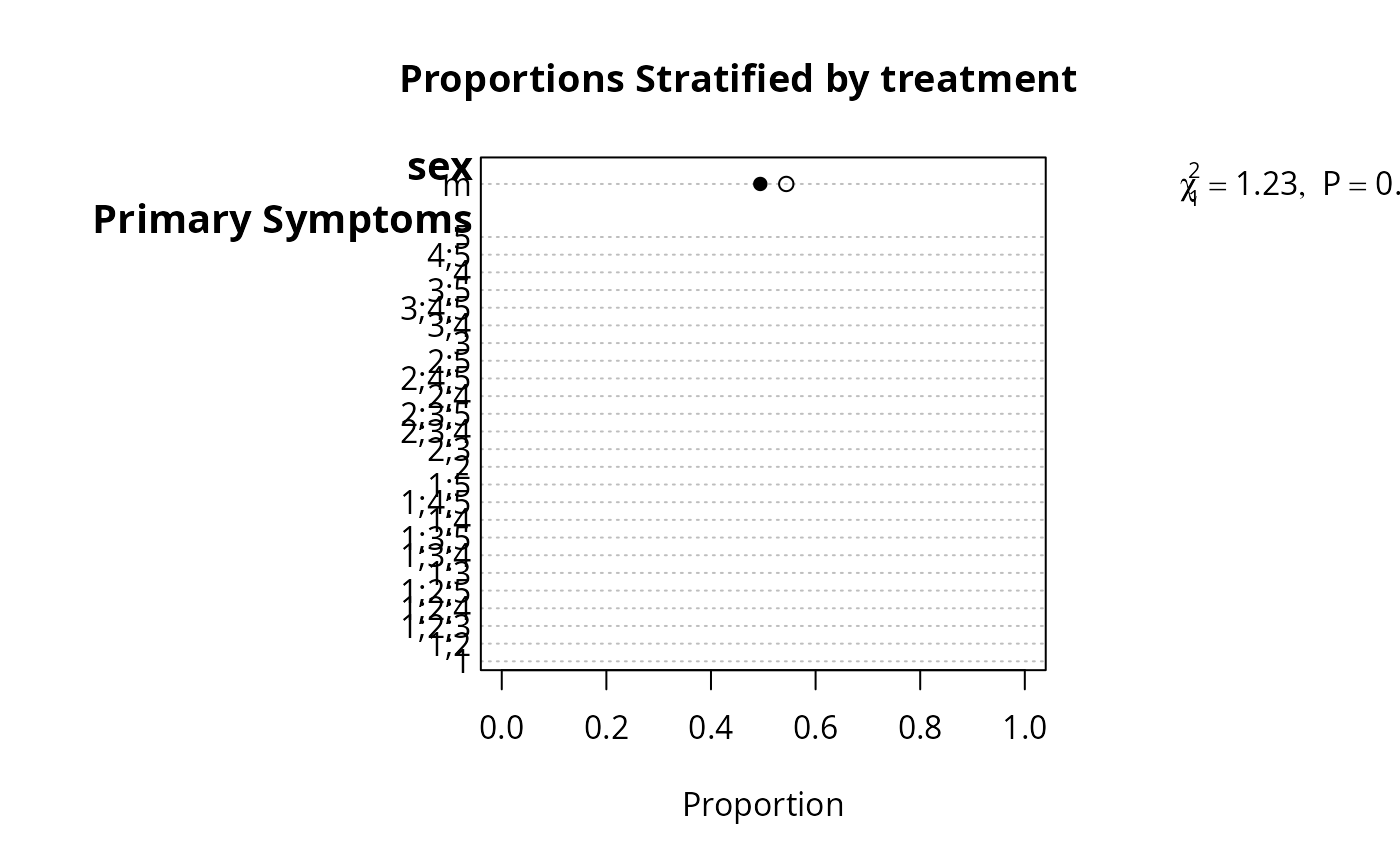
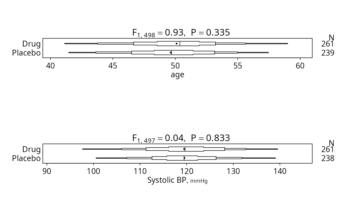
plot(f)    # first specify options(grType='plotly') to use plotly


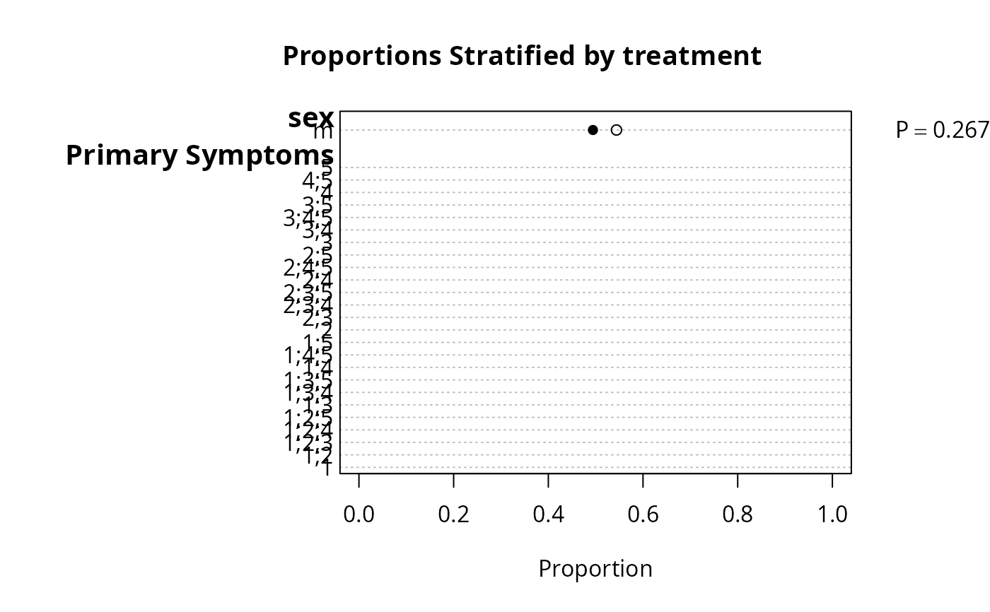
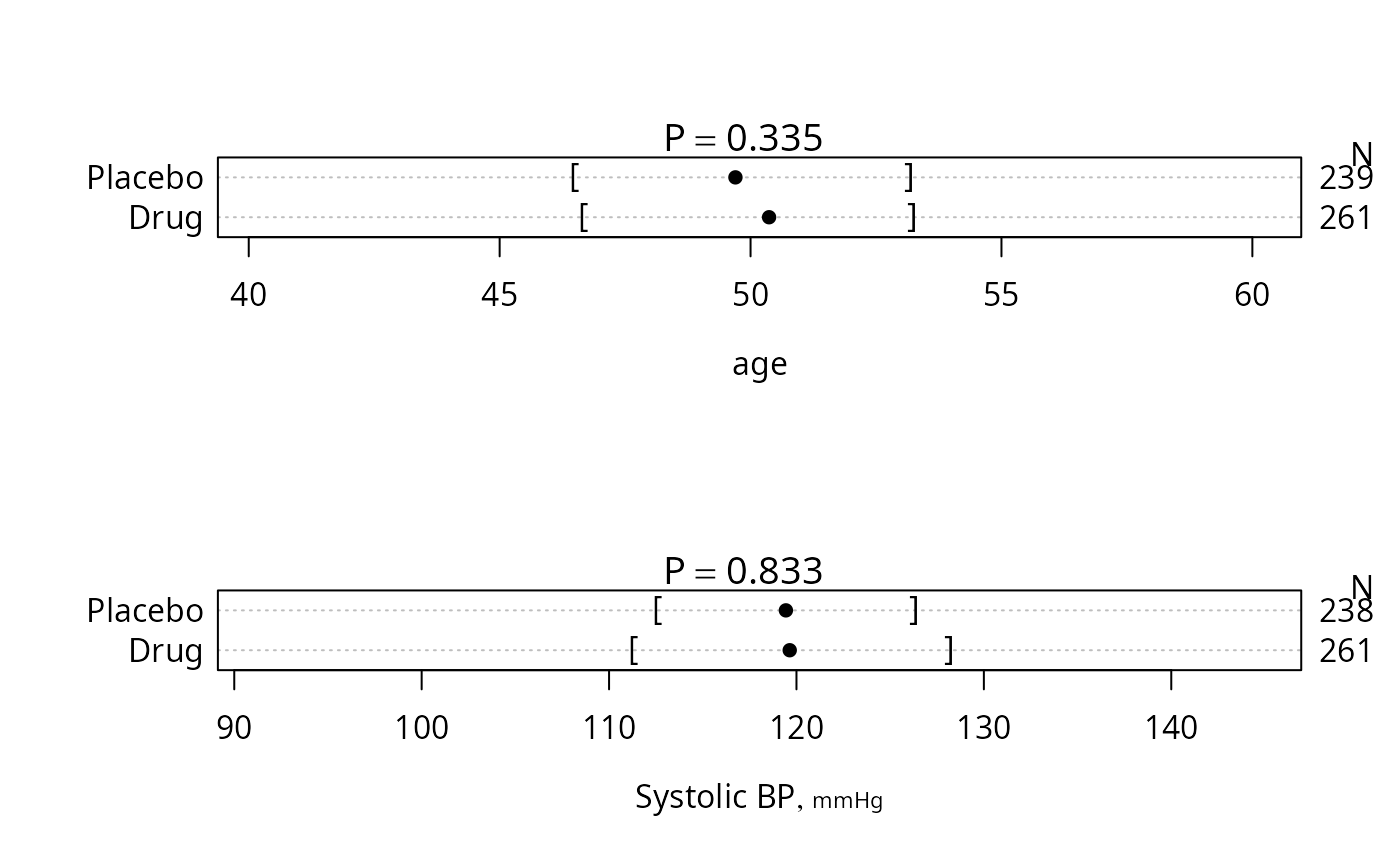
plot(f, conType='dot', prtest='P')


bpplt()    # annotated example showing layout of bp plot


# Produce separate tables by country
f <- summaryM(age + sex + sbp + Symptoms ~ treatment + country,
              groups='treatment', test=TRUE)
f
#> 
#> Canada
#> 
#> 
#> Descriptive Statistics  (N=247)
#> 
#> +--------------------+---+----------------------+----------------------+------------------------------+
#> |                    |N  |Drug                  |Placebo               |  Test                        |
#> |                    |   |(N=124)               |(N=123)               |Statistic                     |
#> +--------------------+---+----------------------+----------------------+------------------------------+
#> |age                 |247|        48.1/51.0/53.3|        47.0/50.1/52.9|   F=3.14 d.f.=1,245 P=0.078  |
#> +--------------------+---+----------------------+----------------------+------------------------------+
#> |sex : m             |247|          0.52  (65)  |          0.56  (69)  |Chi-square=0.34 d.f.=1 P=0.562|
#> +--------------------+---+----------------------+----------------------+------------------------------+
#> |Systolic BP [mmHg]  |247|          111/120/128 |          113/120/127 |   F=0.03 d.f.=1,245 P=0.862  |
#> +--------------------+---+----------------------+----------------------+------------------------------+
#> |Primary Symptoms : 1|  0|                      |                      |                              |
#> +--------------------+---+----------------------+----------------------+------------------------------+
#> |    1;2             |   |                      |                      |                              |
#> +--------------------+---+----------------------+----------------------+------------------------------+
#> |    1;2;3           |   |                      |                      |                              |
#> +--------------------+---+----------------------+----------------------+------------------------------+
#> |    1;2;4           |   |                      |                      |                              |
#> +--------------------+---+----------------------+----------------------+------------------------------+
#> |    1;2;5           |   |                      |                      |                              |
#> +--------------------+---+----------------------+----------------------+------------------------------+
#> |    1;3             |   |                      |                      |                              |
#> +--------------------+---+----------------------+----------------------+------------------------------+
#> |    1;3;4           |   |                      |                      |                              |
#> +--------------------+---+----------------------+----------------------+------------------------------+
#> |    1;3;5           |   |                      |                      |                              |
#> +--------------------+---+----------------------+----------------------+------------------------------+
#> |    1;4             |   |                      |                      |                              |
#> +--------------------+---+----------------------+----------------------+------------------------------+
#> |    1;4;5           |   |                      |                      |                              |
#> +--------------------+---+----------------------+----------------------+------------------------------+
#> |    1;5             |   |                      |                      |                              |
#> +--------------------+---+----------------------+----------------------+------------------------------+
#> |    2               |   |                      |                      |                              |
#> +--------------------+---+----------------------+----------------------+------------------------------+
#> |    2;3             |   |                      |                      |                              |
#> +--------------------+---+----------------------+----------------------+------------------------------+
#> |    2;3;4           |   |                      |                      |                              |
#> +--------------------+---+----------------------+----------------------+------------------------------+
#> |    2;3;5           |   |                      |                      |                              |
#> +--------------------+---+----------------------+----------------------+------------------------------+
#> |    2;4             |   |                      |                      |                              |
#> +--------------------+---+----------------------+----------------------+------------------------------+
#> |    2;4;5           |   |                      |                      |                              |
#> +--------------------+---+----------------------+----------------------+------------------------------+
#> |    2;5             |   |                      |                      |                              |
#> +--------------------+---+----------------------+----------------------+------------------------------+
#> |    3               |   |                      |                      |                              |
#> +--------------------+---+----------------------+----------------------+------------------------------+
#> |    3;4             |   |                      |                      |                              |
#> +--------------------+---+----------------------+----------------------+------------------------------+
#> |    3;4;5           |   |                      |                      |                              |
#> +--------------------+---+----------------------+----------------------+------------------------------+
#> |    3;5             |   |                      |                      |                              |
#> +--------------------+---+----------------------+----------------------+------------------------------+
#> |    4               |   |                      |                      |                              |
#> +--------------------+---+----------------------+----------------------+------------------------------+
#> |    4;5             |   |                      |                      |                              |
#> +--------------------+---+----------------------+----------------------+------------------------------+
#> |    5               |   |                      |                      |                              |
#> +--------------------+---+----------------------+----------------------+------------------------------+
#> 
#> US
#> 
#> 
#> Descriptive Statistics  (N=253)
#> 
#> +--------------------+---+----------------------+----------------------+------------------------------+
#> |                    |N  |Drug                  |Placebo               |  Test                        |
#> |                    |   |(N=137)               |(N=116)               |Statistic                     |
#> +--------------------+---+----------------------+----------------------+------------------------------+
#> |age                 |253|        45.6/49.3/53.1|        46.1/49.3/53.7|   F=0.08 d.f.=1,251 P=0.775  |
#> +--------------------+---+----------------------+----------------------+------------------------------+
#> |sex : m             |253|          0.47  (64)  |          0.53  (61)  |Chi-square=0.87 d.f.=1 P=0.352|
#> +--------------------+---+----------------------+----------------------+------------------------------+
#> |Systolic BP [mmHg]  |252|          111/120/128 |          113/119/126 |    F=0.02 d.f.=1,250 P=0.9   |
#> +--------------------+---+----------------------+----------------------+------------------------------+
#> |Primary Symptoms : 1|  0|                      |                      |                              |
#> +--------------------+---+----------------------+----------------------+------------------------------+
#> |    1;2             |   |                      |                      |                              |
#> +--------------------+---+----------------------+----------------------+------------------------------+
#> |    1;2;3           |   |                      |                      |                              |
#> +--------------------+---+----------------------+----------------------+------------------------------+
#> |    1;2;4           |   |                      |                      |                              |
#> +--------------------+---+----------------------+----------------------+------------------------------+
#> |    1;2;5           |   |                      |                      |                              |
#> +--------------------+---+----------------------+----------------------+------------------------------+
#> |    1;3             |   |                      |                      |                              |
#> +--------------------+---+----------------------+----------------------+------------------------------+
#> |    1;3;4           |   |                      |                      |                              |
#> +--------------------+---+----------------------+----------------------+------------------------------+
#> |    1;3;5           |   |                      |                      |                              |
#> +--------------------+---+----------------------+----------------------+------------------------------+
#> |    1;4             |   |                      |                      |                              |
#> +--------------------+---+----------------------+----------------------+------------------------------+
#> |    1;4;5           |   |                      |                      |                              |
#> +--------------------+---+----------------------+----------------------+------------------------------+
#> |    1;5             |   |                      |                      |                              |
#> +--------------------+---+----------------------+----------------------+------------------------------+
#> |    2               |   |                      |                      |                              |
#> +--------------------+---+----------------------+----------------------+------------------------------+
#> |    2;3             |   |                      |                      |                              |
#> +--------------------+---+----------------------+----------------------+------------------------------+
#> |    2;3;4           |   |                      |                      |                              |
#> +--------------------+---+----------------------+----------------------+------------------------------+
#> |    2;3;5           |   |                      |                      |                              |
#> +--------------------+---+----------------------+----------------------+------------------------------+
#> |    2;4             |   |                      |                      |                              |
#> +--------------------+---+----------------------+----------------------+------------------------------+
#> |    2;4;5           |   |                      |                      |                              |
#> +--------------------+---+----------------------+----------------------+------------------------------+
#> |    2;5             |   |                      |                      |                              |
#> +--------------------+---+----------------------+----------------------+------------------------------+
#> |    3               |   |                      |                      |                              |
#> +--------------------+---+----------------------+----------------------+------------------------------+
#> |    3;4             |   |                      |                      |                              |
#> +--------------------+---+----------------------+----------------------+------------------------------+
#> |    3;4;5           |   |                      |                      |                              |
#> +--------------------+---+----------------------+----------------------+------------------------------+
#> |    3;5             |   |                      |                      |                              |
#> +--------------------+---+----------------------+----------------------+------------------------------+
#> |    4               |   |                      |                      |                              |
#> +--------------------+---+----------------------+----------------------+------------------------------+
#> |    4;5             |   |                      |                      |                              |
#> +--------------------+---+----------------------+----------------------+------------------------------+
#> |    5               |   |                      |                      |                              |
#> +--------------------+---+----------------------+----------------------+------------------------------+

if (FALSE) { # \dontrun{
getHdata(pbc)
s5 <- summaryM(bili + albumin + stage + protime + sex + 
               age + spiders ~ drug, data=pbc)

print(s5, npct='both')
# npct='both' : print both numerators and denominators
plot(s5, which='categorical')
Key(locator(1))  # draw legend at mouse click
par(oma=c(3,0,0,0))  # leave outer margin at bottom
plot(s5, which='continuous')  # see also bpplotM
Key2()           # draw legend at lower left corner of plot
                 # oma= above makes this default key fit the page better

options(digits=3)
w <- latex(s5, npct='both', here=TRUE, file='')

options(grType='plotly')
pbc <- upData(pbc, moveUnits = TRUE)
s <- summaryM(bili + albumin + alk.phos + copper + spiders + sex ~
              drug, data=pbc, test=TRUE)
# Render html
options(prType='html')
s   # invokes print.summaryM
a <- plot(s)
a$Categorical
a$Continuous
plot(s, which='con')
} # }