Multiple Imputation using Additive Regression, Bootstrapping, and Predictive Mean Matching

The transcan function creates flexible additive imputation models but provides only an approximation to true multiple imputation as the imputation models are fixed before all multiple imputations are drawn. This ignores variability caused by having to fit the imputation models. aregImpute takes all aspects of uncertainty in the imputations into account by using the bootstrap to approximate the process of drawing predicted values from a full Bayesian predictive distribution. Different bootstrap resamples are used for each of the multiple imputations, i.e., for the ith imputation of a sometimes missing variable, i=1,2,... n.impute, a flexible additive model is fitted on a sample with replacement from the original data and this model is used to predict all of the original missing and non-missing values for the target variable.

areg is used to fit the imputation models. By default, linearity is assumed for target variables (variables being imputed) and nk=3 knots are assumed for continuous predictors transformed using restricted cubic splines. If nk is three or greater and tlinear is set to FALSE, areg simultaneously finds transformations of the target variable and of all of the predictors, to get a good fit assuming additivity, maximizing $R^2$, using the same canonical correlation method as transcan. Flexible transformations may be overridden for specific variables by specifying the identity transformation for them. When a categorical variable is being predicted, the flexible transformation is Fisher's optimum scoring method. Nonlinear transformations for continuous variables may be nonmonotonic. If nk is a vector, areg's bootstrap and crossval=10 options will be used to help find the optimum validating value of nk over values of that vector, at the last imputation iteration. For the imputations, the minimum value of nk is used.

Instead of defaulting to taking random draws from fitted imputation models using random residuals as is done by transcan, aregImpute by default uses predictive mean matching with optional weighted probability sampling of donors rather than using only the closest match. Predictive mean matching works for binary, categorical, and continuous variables without the need for iterative maximum likelihood fitting for binary and categorical variables, and without the need for computing residuals or for curtailing imputed values to be in the range of actual data. Predictive mean matching is especially attractive when the variable being imputed is also being transformed automatically. Constraints may be placed on variables being imputed with predictive mean matching, e.g., a missing hospital discharge date may be required to be imputed from a donor observation whose discharge date is before the recipient subject's first post-discharge visit date. See Details below for more information about the algorithm. A "regression" method is also available that is similar to that used in transcan. This option should be used when mechanistic missingness requires the use of extrapolation during imputation.

A print method summarizes the results, and a plot method plots distributions of imputed values. Typically, fit.mult.impute will be called after aregImpute.

If a target variable is transformed nonlinearly (i.e., if nk is greater than zero and tlinear is set to FALSE) and the estimated target variable transformation is non-monotonic, imputed values are not unique. When type='regression', a random choice of possible inverse values is made.

The reformM function provides two ways of recreating a formula to give to aregImpute by reordering the variables in the formula. This is a modified version of a function written by Yong Hao Pua. One can specify nperm to obtain a list of nperm randomly permuted variables. The list is converted to a single ordinary formula if nperm=1. If nperm is omitted, variables are sorted in descending order of the number of NAs. reformM also prints a recommended number of multiple imputations to use, which is a minimum of 5 and the percent of incomplete observations.

Usage

aregImpute(formula, data, subset, n.impute=5, group=NULL,
           nk=3, tlinear=TRUE, type=c('pmm','regression','normpmm'),
           pmmtype=1, match=c('weighted','closest','kclosest'),
           kclosest=3, fweighted=0.2,
           curtail=TRUE, constraint=NULL,
           boot.method=c('simple', 'approximate bayesian'),
           burnin=3, x=FALSE, pr=TRUE, plotTrans=FALSE, tolerance=NULL, B=75)
# S3 method for class 'aregImpute'
print(x, digits=3, ...)
# S3 method for class 'aregImpute'
plot(x, nclass=NULL, type=c('ecdf','hist'),
     datadensity=c("hist", "none", "rug", "density"),
     diagnostics=FALSE, maxn=10, ...)
reformM(formula, data, nperm)

Arguments

formula: an S model formula. You can specify restrictions for transformations of variables. The function automatically determines which variables are categorical (i.e., factor, category, or character vectors). Binary variables are automatically restricted to be linear. Force linear transformations of continuous variables by enclosing variables by the identify function (I()). It is recommended that factor() or as.factor() do not appear in the formula but instead variables be converted to factors as needed and stored in the data frame. That way imputations for factor variables (done using impute.transcan for example) will be correct. Currently reformM does not handle variables that are enclosed in functions such as I().
x: an object created by aregImpute. For aregImpute, set x to TRUE to save the data matrix containing the final (number n.impute) imputations in the result. This is needed if you want to later do out-of-sample imputation. Categorical variables are coded as integers in this matrix.
data: input raw data
subset: These may be also be specified. You may not specify na.action as na.retain is always used.
n.impute: number of multiple imputations. n.impute=5 is frequently recommended but 10 or more doesn't hurt.
group: a character or factor variable the same length as the number of observations in data and containing no NAs. When group is present, causes a bootstrap sample of the observations corresponding to non-NAs of a target variable to have the same frequency distribution of group as the that in the non-NAs of the original sample. This can handle k-sample problems as well as lower the chance that a bootstrap sample will have a missing cell when the original cell frequency was low.
nk: number of knots to use for continuous variables. When both the target variable and the predictors are having optimum transformations estimated, there is more instability than with normal regression so the complexity of the model should decrease more sharply as the sample size decreases. Hence set nk to 0 (to force linearity for non-categorical variables) or 3 (minimum number of knots possible with a linear tail-restricted cubic spline) for small sample sizes. Simulated problems as in the examples section can assist in choosing nk. Set nk to a vector to get bootstrap-validated and 10-fold cross-validated $R^2$ and mean and median absolute prediction errors for imputing each sometimes-missing variable, with nk ranging over the given vector. The errors are on the original untransformed scale. The mean absolute error is the recommended basis for choosing the number of knots (or linearity).
tlinear: set to FALSE to allow a target variable (variable being imputed) to have a nonlinear left-hand-side transformation when nk is 3 or greater
type: The default is "pmm" for predictive mean matching, which is a more nonparametric approach that will work for categorical as well as continuous predictors. Alternatively, use "regression" when all variables that are sometimes missing are continuous and the missingness mechanism is such that entire intervals of population values are unobserved. See the Details section for more information. Another method, type="normpmm", only works when variables containing NAs are continuous and tlinear is TRUE (the default), meaning that the variable being imputed is not transformed when it is on the left hand model side. normpmm assumes that the imputation regression parameter estimates are multivariately normally distributed and that the residual variance has a scaled chi-squared distribution. For each imputation a random draw of the estimates is taken and a random draw from sigma is combined with those to get a random draw from the posterior predicted value distribution. Predictive mean matching is then done matching these predicted values from incomplete observations with predicted values from complete potential donor observations, where the latter predictions are based on the imputation model least squares parameter estimates and not on random draws from the posterior. For the plot method, specify type="hist" to draw histograms of imputed values with rug plots at the top, or type="ecdf" (the default) to draw empirical CDFs with spike histograms at the bottom.
pmmtype: type of matching to be used for predictive mean matching when type="pmm". pmmtype=2 means that predicted values for both target incomplete and complete observations come from a fit from the same bootstrap sample. pmmtype=1, the default, means that predicted values for complete observations are based on additive regression fits on original complete observations (using last imputations for non-target variables as with the other methds), and using fits on a bootstrap sample to get predicted values for missing target variables. See van Buuren (2012) section 3.4.2 where pmmtype=1 is said to work much better when the number of variables is small. pmmtype=3 means that complete observation predicted values come from a bootstrap sample fit whereas target incomplete observation predicted values come from a sample with replacement from the bootstrap fit (approximate Bayesian bootstrap).
match: Defaults to match="weighted" to do weighted multinomial probability sampling using the tricube function (similar to lowess) as the weights. The argument of the tricube function is the absolute difference in transformed predicted values of all the donors and of the target predicted value, divided by a scaling factor. The scaling factor in the tricube function is fweighted times the mean absolute difference between the target predicted value and all the possible donor predicted values. Set match="closest" to find as the donor the observation having the closest predicted transformed value, even if that same donor is found repeatedly. Set match="kclosest" to use a slower implementation that finds, after jittering the complete case predicted values, the kclosest complete cases on the target variable being imputed, then takes a random sample of one of these kclosest cases.
kclosest: see match
fweighted: Smoothing parameter (multiple of mean absolute difference) used when match="weighted", with a default value of 0.2. Set fweighted to a number between 0.02 and 0.2 to force the donor to have a predicted value closer to the target, and set fweighted to larger values (but seldom larger than 1.0) to allow donor values to be less tightly matched. See the examples below to learn how to study the relationship between fweighted and the standard deviation of multiple imputations within individuals.
curtail: applies if type='regression', causing imputed values to be curtailed at the observed range of the target variable. Set to FALSE to allow extrapolation outside the data range.
constraint: for predictive mean matching constraint is a named list specifying R expression()s encoding constaints on which donor observations are allowed to be used, based on variables that are not missing, i.e., based on donor observations and/or recipient observations as long as the target variable being imputed is not used for the recipients. The expressions must evaluate to a logical vector with no NAs and whose length is the number of rows in the donor observations. The expressions refer to donor observations by prefixing variable names by d$, and to a single recipient observation by prefixing variables names by r$.
boot.method: By default, simple boostrapping is used in which the target variable is predicted using a sample with replacement from the observations with non-missing target variable. Specify boot.method='approximate bayesian' to build the imputation models from a sample with replacement from a sample with replacement of the observations with non-missing targets. Preliminary simulations have shown this results in good confidence coverage of the final model parameters when type='regression' is used. Not implemented when group is used.
burnin: aregImpute does burnin + n.impute iterations of the entire modeling process. The first burnin imputations are discarded. More burn-in iteractions may be requied when multiple variables are missing on the same observations. When only one variable is missing, no burn-ins are needed and burnin is set to zero if unspecified.
pr: set to FALSE to suppress printing of iteration messages
plotTrans: set to TRUE to plot ace or avas transformations for each variable for each of the multiple imputations. This is useful for determining whether transformations are reasonable. If transformations are too noisy or have long flat sections (resulting in "lumps" in the distribution of imputed values), it may be advisable to place restrictions on the transformations (monotonicity or linearity).
tolerance: singularity criterion; list the source code in the lm.fit.qr.bare function for details
B: number of bootstrap resamples to use if nk is a vector
digits: number of digits for printing
nclass: number of bins to use in drawing histogram
datadensity: see Ecdf
diagnostics: Specify diagnostics=TRUE to draw plots of imputed values against sequential imputation numbers, separately for each missing observations and variable.
maxn: Maximum number of observations shown for diagnostics. Default is maxn=10, which limits the number of observations plotted to at most the first 10.
nperm: number of random formula permutations for reformM; omit to sort variables by descending missing count.
...: other arguments that are ignored

Value

a list of class "aregImpute" containing the following elements:

call: the function call expression
formula: the formula specified to aregImpute
match: the match argument
fweighted: the fweighted argument
n: total number of observations in input dataset
p: number of variables
na: list of subscripts of observations for which values were originally missing
nna: named vector containing the numbers of missing values in the data
type: vector of types of transformations used for each variable ("s","l","c" for smooth spline, linear, or categorical with dummy variables)
tlinear: value of tlinear parameter
nk: number of knots used for smooth transformations
cat.levels: list containing character vectors specifying the levels of categorical variables
df: degrees of freedom (number of parameters estimated) for each variable
n.impute: number of multiple imputations per missing value
imputed: a list containing matrices of imputed values in the same format as those created by transcan. Categorical variables are coded using their integer codes. Variables having no missing values will have NULL matrices in the list.
x: if x is TRUE, the original data matrix with integer codes for categorical variables
rsq: for the last round of imputations, a vector containing the R-squares with which each sometimes-missing variable could be predicted from the others by ace or avas.

Details

The sequence of steps used by the aregImpute algorithm is the following.
(1) For each variable containing m NAs where m > 0, initialize the NAs to values from a random sample (without replacement if a sufficient number of non-missing values exist) of size m from the non-missing values.
(2) For burnin+n.impute iterations do the following steps. The first burnin iterations provide a burn-in, and imputations are saved only from the last n.impute iterations.
(3) For each variable containing any NAs, draw a sample with replacement from the observations in the entire dataset in which the current variable being imputed is non-missing. Fit a flexible additive model to predict this target variable while finding the optimum transformation of it (unless the identity transformation is forced). Use this fitted flexible model to predict the target variable in all of the original observations. Impute each missing value of the target variable with the observed value whose predicted transformed value is closest to the predicted transformed value of the missing value (if match="closest" and type="pmm"), or use a draw from a multinomial distribution with probabilities derived from distance weights, if match="weighted" (the default).
(4) After these imputations are computed, use these random draw imputations the next time the curent target variable is used as a predictor of other sometimes-missing variables.

When match="closest", predictive mean matching does not work well when fewer than 3 variables are used to predict the target variable, because many of the multiple imputations for an observation will be identical. In the extreme case of one right-hand-side variable and assuming that only monotonic transformations of left and right-side variables are allowed, every bootstrap resample will give predicted values of the target variable that are monotonically related to predicted values from every other bootstrap resample. The same is true for Bayesian predicted values. This causes predictive mean matching to always match on the same donor observation.

When the missingness mechanism for a variable is so systematic that the distribution of observed values is truncated, predictive mean matching does not work. It will only yield imputed values that are near observed values, so intervals in which no values are observed will not be populated by imputed values. For this case, the only hope is to make regression assumptions and use extrapolation. With type="regression", aregImpute will use linear extrapolation to obtain a (hopefully) reasonable distribution of imputed values. The "regression" option causes aregImpute to impute missing values by adding a random sample of residuals (with replacement if there are more NAs than measured values) on the transformed scale of the target variable. After random residuals are added, predicted random draws are obtained on the original untransformed scale using reverse linear interpolation on the table of original and transformed target values (linear extrapolation when a random residual is large enough to put the random draw prediction outside the range of observed values). The bootstrap is used as with type="pmm" to factor in the uncertainty of the imputation model.

As model uncertainty is high when the transformation of a target variable is unknown, tlinear defaults to TRUE to limit the variance in predicted values when nk is positive.

Author

Frank Harrell
Department of Biostatistics
Vanderbilt University
fh@fharrell.com

References

van Buuren, Stef. Flexible Imputation of Missing Data. Chapman & Hall/CRC, Boca Raton FL, 2012.

Little R, An H. Robust likelihood-based analysis of multivariate data with missing values. Statistica Sinica 14:949-968, 2004.

van Buuren S, Brand JPL, Groothuis-Oudshoorn CGM, Rubin DB. Fully conditional specifications in multivariate imputation. J Stat Comp Sim 72:1049-1064, 2006.

de Groot JAH, Janssen KJM, Zwinderman AH, Moons KGM, Reitsma JB. Multiple imputation to correct for partial verification bias revisited. Stat Med 27:5880-5889, 2008.

Siddique J. Multiple imputation using an iterative hot-deck with distance-based donor selection. Stat Med 27:83-102, 2008.

White IR, Royston P, Wood AM. Multiple imputation using chained equations: Issues and guidance for practice. Stat Med 30:377-399, 2011.

Curnow E, Carpenter JR, Heron JE, et al: Multiple imputation of missing data under missing at random: compatible imputation models are not sufficient to avoid bias if they are mis-specified. J Clin Epi June 9, 2023. DOI:10.1016/j.jclinepi.2023.06.011.

Examples

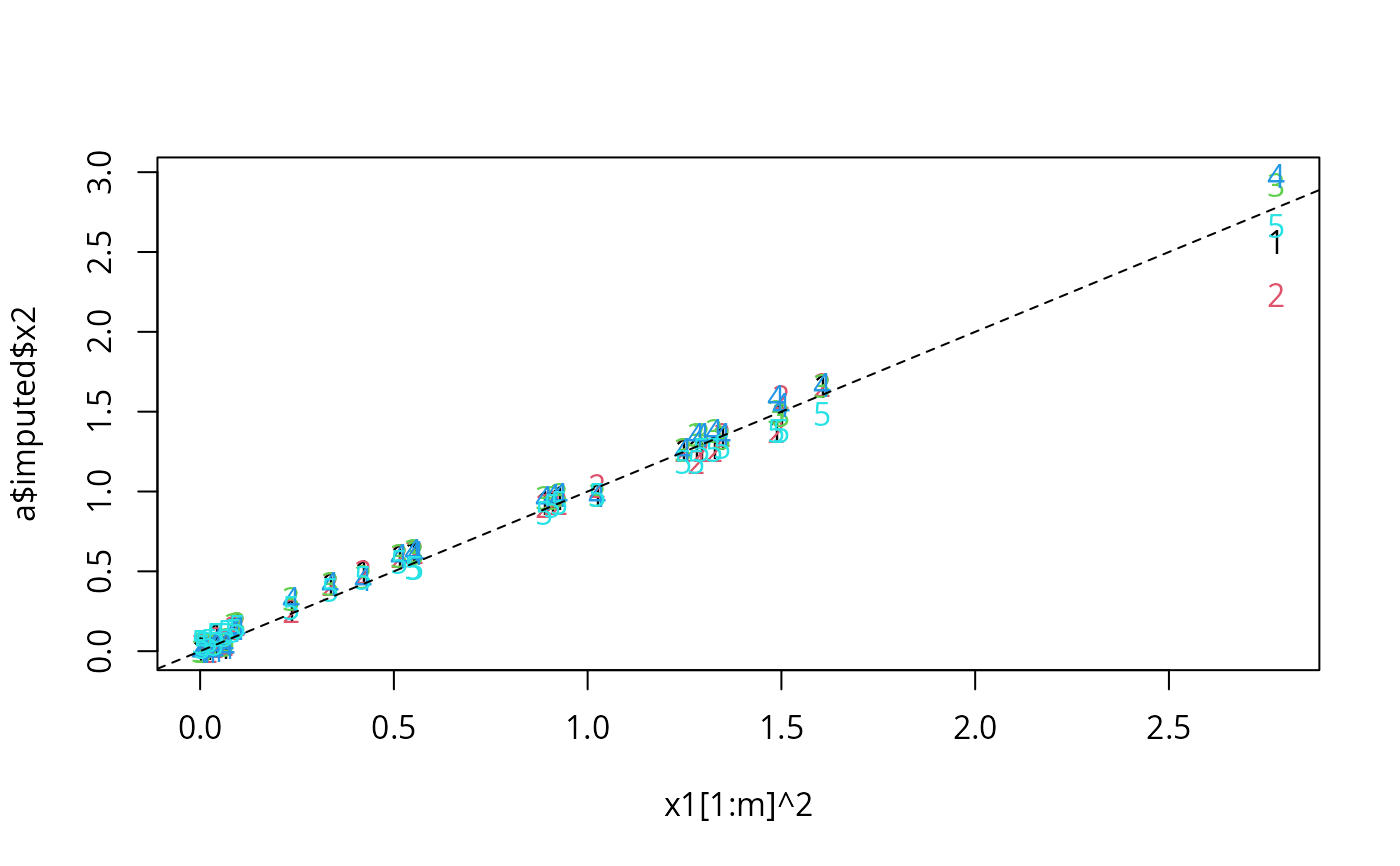
# Check that aregImpute can almost exactly estimate missing values when
# there is a perfect nonlinear relationship between two variables
# Fit restricted cubic splines with 4 knots for x1 and x2, linear for x3
set.seed(3)
x1 <- rnorm(200)
x2 <- x1^2
x3 <- runif(200)
m <- 30
x2[1:m] <- NA
a <- aregImpute(~x1+x2+I(x3), n.impute=5, nk=4, match='closest')
#> Iteration 1 
Iteration 2 
Iteration 3 
Iteration 4 
Iteration 5 

a
#> 
#> Multiple Imputation using Bootstrap and PMM
#> 
#> aregImpute(formula = ~x1 + x2 + I(x3), n.impute = 5, nk = 4, 
#>     match = "closest")
#> 
#> n: 200 	p: 3 	Imputations: 5  	nk: 4 
#> 
#> Number of NAs:
#> x1 x2 x3 
#>  0 30  0 
#> 
#>    type d.f.
#> x1    s    3
#> x2    s    1
#> x3    l    1
#> 
#> Transformation of Target Variables Forced to be Linear
#> 
#> R-squares for Predicting Non-Missing Values for Each Variable
#> Using Last Imputations of Predictors
#>    x2 
#> 0.984 
matplot(x1[1:m]^2, a$imputed$x2)
abline(a=0, b=1, lty=2)


x1[1:m]^2
#>  [1] 0.925315897 0.085571299 0.066971341 1.327407883 0.038330915 0.000907452
#>  [7] 0.007296189 1.246818367 1.485613400 1.606223478 0.554699626 1.279655455
#> [13] 0.513169486 0.063833220 0.023117897 0.094652479 0.908242033 0.420218743
#> [19] 1.498943851 0.039924679 0.334643416 0.887930672 0.041505171 2.777138392
#> [25] 0.234696753 0.549188688 1.347028987 1.024279865 0.005195306 1.292273993
a$imputed$x2
#>           [,1]        [,2]         [,3]         [,4]       [,5]
#> 1  0.958996702 0.930577069 9.762484e-01 9.799896e-01 0.93057707
#> 2  0.149052972 0.146963621 1.661947e-01 1.353046e-01 0.12388046
#> 3  0.056748811 0.056748811 7.148054e-02 2.631055e-02 0.12140884
#> 4  1.278855629 1.262597928 1.379068e+00 1.379068e+00 1.26259793
#> 5  0.035671951 0.035671951 4.655437e-02 3.567195e-02 0.04379575
#> 6  0.004982439 0.035671951 1.463217e-03 4.099071e-05 0.05595187
#> 7  0.035671951 0.034669484 4.099071e-05 4.099071e-05 0.04379575
#> 8  1.262597928 1.262597928 1.262598e+00 1.262598e+00 1.18470752
#> 9  1.379068228 1.379068228 1.499170e+00 1.591427e+00 1.37906823
#> 10 1.661538043 1.667583069 1.661538e+00 1.667583e+00 1.48316856
#> 11 0.618593060 0.618593060 6.164482e-01 6.164482e-01 0.51992134
#> 12 1.262597928 1.184707523 1.355782e+00 1.354657e+00 1.18470752
#> 13 0.594890076 0.594890076 5.948901e-01 5.948901e-01 0.55889449
#> 14 0.026310553 0.046554372 3.883560e-02 5.108231e-02 0.10438988
#> 15 0.020493742 0.002514871 3.466948e-02 2.514871e-03 0.06568317
#> 16 0.166194673 0.168263518 1.682635e-01 1.469636e-01 0.14905297
#> 17 0.930577069 0.930577069 9.589967e-01 9.698616e-01 0.91224047
#> 18 0.497752140 0.497752140 4.659193e-01 4.505450e-01 0.45543010
#> 19 1.479656909 1.591426720 1.479657e+00 1.543022e+00 1.37906823
#> 20 0.042739772 0.034669484 4.273977e-02 4.982439e-03 0.10438988
#> 21 0.422393723 0.422393723 4.223937e-01 4.223937e-01 0.38112108
#> 22 0.930577069 0.912240467 9.589967e-01 9.589967e-01 0.86794372
#> 23 0.104389875 0.078255416 4.379575e-02 7.133446e-02 0.10438988
#> 24 2.562633045 2.228492325 2.921218e+00 2.973363e+00 2.66392498
#> 25 0.250603132 0.250603132 3.289231e-01 3.289231e-01 0.26743794
#> 26 0.618593060 0.618593060 6.300569e-01 6.300569e-01 0.51992134
#> 27 1.337073813 1.354657372 1.337074e+00 1.355782e+00 1.27885563
#> 28 0.980088775 1.035227246 9.799896e-01 9.799896e-01 0.97998959
#> 29 0.034669484 0.034669484 4.273977e-02 1.634461e-02 0.02460284
#> 30 1.262597928 1.262597928 1.355782e+00 1.354657e+00 1.26259793


# Multiple imputation and estimation of variances and covariances of
# regression coefficient estimates accounting for imputation
# Example 1: large sample size, much missing data, no overlap in
# NAs across variables
x1 <- factor(sample(c('a','b','c'),1000,TRUE))
x2 <- (x1=='b') + 3*(x1=='c') + rnorm(1000,0,2)
x3 <- rnorm(1000)
y  <- x2 + 1*(x1=='c') + .2*x3 + rnorm(1000,0,2)
orig.x1 <- x1[1:250]
orig.x2 <- x2[251:350]
x1[1:250] <- NA
x2[251:350] <- NA
d <- data.frame(x1,x2,x3,y, stringsAsFactors=TRUE)
# Find value of nk that yields best validating imputation models
# tlinear=FALSE means to not force the target variable to be linear
f <- aregImpute(~y + x1 + x2 + x3, nk=c(0,3:5), tlinear=FALSE,
                data=d, B=10) # normally B=75
#> Iteration 1 
Iteration 2 
Iteration 3 
Iteration 4 
Iteration 5 
Iteration 6 
Iteration 7 
Iteration 8 

f
#> 
#> Multiple Imputation using Bootstrap and PMM
#> 
#> aregImpute(formula = ~y + x1 + x2 + x3, data = d, nk = c(0, 3:5), 
#>     tlinear = FALSE, B = 10)
#> 
#> n: 1000 	p: 4 	Imputations: 5  	nk: 0 
#> 
#> Number of NAs:
#>   y  x1  x2  x3 
#>   0 250 100   0 
#> 
#>    type d.f.
#> y     s    1
#> x1    c    2
#> x2    s    1
#> x3    s    1
#> 
#> R-squares for Predicting Non-Missing Values for Each Variable
#> Using Last Imputations of Predictors
#>    x1    x2 
#> 0.331 0.611 
#> 
#> Resampling results for determining the complexity of imputation models
#> 
#> Variable being imputed: x1 
#>                                          nk=0  nk=3  nk=4  nk=5
#> Bootstrap bias-corrected R^2            0.327 0.332 0.351 0.346
#> 10-fold cross-validated  R^2            0.340 0.351 0.351 0.342
#> Bootstrap bias-corrected mean   |error| 1.072 1.069 1.062 1.067
#> 10-fold cross-validated  mean   |error| 0.489 0.486 0.494 0.498
#> Bootstrap bias-corrected median |error| 1.000 1.000 1.000 1.000
#> 10-fold cross-validated  median |error| 0.000 0.200 0.000 0.200
#> 
#> Variable being imputed: x2 
#>                                          nk=0  nk=3  nk=4  nk=5
#> Bootstrap bias-corrected R^2            0.652 0.638 0.635 0.647
#> 10-fold cross-validated  R^2            0.635 0.643 0.635 0.634
#> Bootstrap bias-corrected mean   |error| 1.140 1.196 1.200 1.193
#> 10-fold cross-validated  mean   |error| 1.712 1.203 1.202 1.202
#> Bootstrap bias-corrected median |error| 0.984 0.962 0.997 0.985
#> 10-fold cross-validated  median |error| 1.436 0.980 1.007 0.995
#> 
#> 
# Try forcing target variable (x1, then x2) to be linear while allowing
# predictors to be nonlinear (could also say tlinear=TRUE)
f <- aregImpute(~y + x1 + x2 + x3, nk=c(0,3:5), data=d, B=10)
#> Iteration 1 
Iteration 2 
Iteration 3 
Iteration 4 
Iteration 5 
Iteration 6 
Iteration 7 
Iteration 8 

f
#> 
#> Multiple Imputation using Bootstrap and PMM
#> 
#> aregImpute(formula = ~y + x1 + x2 + x3, data = d, nk = c(0, 3:5), 
#>     B = 10)
#> 
#> n: 1000 	p: 4 	Imputations: 5  	nk: 0 
#> 
#> Number of NAs:
#>   y  x1  x2  x3 
#>   0 250 100   0 
#> 
#>    type d.f.
#> y     s    1
#> x1    c    2
#> x2    s    1
#> x3    s    1
#> 
#> Transformation of Target Variables Forced to be Linear
#> 
#> R-squares for Predicting Non-Missing Values for Each Variable
#> Using Last Imputations of Predictors
#>    x1    x2 
#> 0.358 0.621 
#> 
#> Resampling results for determining the complexity of imputation models
#> 
#> Variable being imputed: x1 
#>                                          nk=0  nk=3  nk=4  nk=5
#> Bootstrap bias-corrected R^2            0.334 0.336 0.341 0.342
#> 10-fold cross-validated  R^2            0.329 0.334 0.337 0.336
#> Bootstrap bias-corrected mean   |error| 1.058 1.061 1.052 1.052
#> 10-fold cross-validated  mean   |error| 0.492 0.486 0.485 0.488
#> Bootstrap bias-corrected median |error| 1.000 1.000 1.000 1.000
#> 10-fold cross-validated  median |error| 0.100 0.300 0.100 0.100
#> 
#> Variable being imputed: x2 
#>                                          nk=0  nk=3  nk=4  nk=5
#> Bootstrap bias-corrected R^2            0.633 0.631 0.635 0.618
#> 10-fold cross-validated  R^2            0.629 0.629 0.626 0.627
#> Bootstrap bias-corrected mean   |error| 1.165 1.168 1.174 1.199
#> 10-fold cross-validated  mean   |error| 1.736 1.731 1.742 1.737
#> Bootstrap bias-corrected median |error| 1.005 1.007 1.010 1.020
#> 10-fold cross-validated  median |error| 1.450 1.445 1.454 1.464
#> 
#> 

if (FALSE) { # \dontrun{
# Use 100 imputations to better check against individual true values
f <- aregImpute(~y + x1 + x2 + x3, n.impute=100, data=d)
f
par(mfrow=c(2,1))
plot(f)
modecat <- function(u) {
 tab <- table(u)
 as.numeric(names(tab)[tab==max(tab)][1])
}
table(orig.x1,apply(f$imputed$x1, 1, modecat))
par(mfrow=c(1,1))
plot(orig.x2, apply(f$imputed$x2, 1, mean))
fmi <- fit.mult.impute(y ~ x1 + x2 + x3, lm, f, 
                       data=d)
sqrt(diag(vcov(fmi)))
fcc <- lm(y ~ x1 + x2 + x3)
summary(fcc)   # SEs are larger than from mult. imputation
} # }
if (FALSE) { # \dontrun{
# Example 2: Very discriminating imputation models,
# x1 and x2 have some NAs on the same rows, smaller n
set.seed(5)
x1 <- factor(sample(c('a','b','c'),100,TRUE))
x2 <- (x1=='b') + 3*(x1=='c') + rnorm(100,0,.4)
x3 <- rnorm(100)
y  <- x2 + 1*(x1=='c') + .2*x3 + rnorm(100,0,.4)
orig.x1 <- x1[1:20]
orig.x2 <- x2[18:23]
x1[1:20] <- NA
x2[18:23] <- NA
#x2[21:25] <- NA
d <- data.frame(x1,x2,x3,y, stringsAsFactors=TRUE)
n <- naclus(d)
plot(n); naplot(n)  # Show patterns of NAs
# 100 imputations to study them; normally use 5 or 10
f  <- aregImpute(~y + x1 + x2 + x3, n.impute=100, nk=0, data=d)
par(mfrow=c(2,3))
plot(f, diagnostics=TRUE, maxn=2)
# Note: diagnostics=TRUE makes graphs similar to those made by:
# r <- range(f$imputed$x2, orig.x2)
# for(i in 1:6) {  # use 1:2 to mimic maxn=2
#   plot(1:100, f$imputed$x2[i,], ylim=r,
#        ylab=paste("Imputations for Obs.",i))
#   abline(h=orig.x2[i],lty=2)
# }

table(orig.x1,apply(f$imputed$x1, 1, modecat))
par(mfrow=c(1,1))
plot(orig.x2, apply(f$imputed$x2, 1, mean))


fmi <- fit.mult.impute(y ~ x1 + x2, lm, f, 
                       data=d)
sqrt(diag(vcov(fmi)))
fcc <- lm(y ~ x1 + x2)
summary(fcc)   # SEs are larger than from mult. imputation
} # }

if (FALSE) { # \dontrun{
# Study relationship between smoothing parameter for weighting function
# (multiplier of mean absolute distance of transformed predicted
# values, used in tricube weighting function) and standard deviation
# of multiple imputations.  SDs are computed from average variances
# across subjects.  match="closest" same as match="weighted" with
# small value of fweighted.
# This example also shows problems with predicted mean
# matching almost always giving the same imputed values when there is
# only one predictor (regression coefficients change over multiple
# imputations but predicted values are virtually 1-1 functions of each
# other)

set.seed(23)
x <- runif(200)
y <- x + runif(200, -.05, .05)
r <- resid(lsfit(x,y))
rmse <- sqrt(sum(r^2)/(200-2))   # sqrt of residual MSE

y[1:20] <- NA
d <- data.frame(x,y)
f <- aregImpute(~ x + y, n.impute=10, match='closest', data=d)
# As an aside here is how to create a completed dataset for imputation
# number 3 as fit.mult.impute would do automatically.  In this degenerate
# case changing 3 to 1-2,4-10 will not alter the results.
imputed <- impute.transcan(f, imputation=3, data=d, list.out=TRUE,
                           pr=FALSE, check=FALSE)
sd <- sqrt(mean(apply(f$imputed$y, 1, var)))

ss <- c(0, .01, .02, seq(.05, 1, length=20))
sds <- ss; sds[1] <- sd

for(i in 2:length(ss)) {
  f <- aregImpute(~ x + y, n.impute=10, fweighted=ss[i])
  sds[i] <- sqrt(mean(apply(f$imputed$y, 1, var)))
}

plot(ss, sds, xlab='Smoothing Parameter', ylab='SD of Imputed Values',
     type='b')
abline(v=.2,  lty=2)  # default value of fweighted
abline(h=rmse, lty=2)  # root MSE of residuals from linear regression
} # }

if (FALSE) { # \dontrun{
# Do a similar experiment for the Titanic dataset
getHdata(titanic3)
h <- lm(age ~ sex + pclass + survived, data=titanic3)
rmse <- summary(h)$sigma
set.seed(21)
f <- aregImpute(~ age + sex + pclass + survived, n.impute=10,
                data=titanic3, match='closest')
sd <- sqrt(mean(apply(f$imputed$age, 1, var)))

ss <- c(0, .01, .02, seq(.05, 1, length=20))
sds <- ss; sds[1] <- sd

for(i in 2:length(ss)) {
  f <- aregImpute(~ age + sex + pclass + survived, data=titanic3,
                  n.impute=10, fweighted=ss[i])
  sds[i] <- sqrt(mean(apply(f$imputed$age, 1, var)))
}

plot(ss, sds, xlab='Smoothing Parameter', ylab='SD of Imputed Values',
     type='b')
abline(v=.2,   lty=2)  # default value of fweighted
abline(h=rmse, lty=2)  # root MSE of residuals from linear regression
} # }


set.seed(2)
d <- data.frame(x1=runif(50), x2=c(rep(NA, 10), runif(40)),
                x3=c(runif(4), rep(NA, 11), runif(35)))
reformM(~ x1 + x2 + x3, data=d)
#> Recommended number of imputations: 30 
#> ~x3 + x2 + x1
#> <environment: 0x5e2f80e9df28>
reformM(~ x1 + x2 + x3, data=d, nperm=2)
#> Recommended number of imputations: 30 
#> [[1]]
#> ~x1 + x2 + x3
#> <environment: 0x5e2f80dd6890>
#> 
#> [[2]]
#> ~x1 + x3 + x2
#> <environment: 0x5e2f80dd6890>
#> 
# Give result or one of the results as the first argument to aregImpute

# Constrain imputed values for two variables
# Require imputed values for x2 to be above 0.2
# Assume x1 is never missing and require imputed values for
# x3 to be less than the recipient's value of x1
a <- aregImpute(~ x1 + x2 + x3, data=d,
                constraint=list(x2 = expression(d$x2 > 0.2),
                                x3 = expression(d$x3 < r$x1)))
#> Iteration 1 
Iteration 2 
Iteration 3 
Iteration 4 
Iteration 5 
Iteration 6 
Iteration 7 
Iteration 8 

a
#> 
#> Multiple Imputation using Bootstrap and PMM
#> 
#> aregImpute(formula = ~x1 + x2 + x3, data = d, constraint = list(x2 = expression(d$x2 > 
#>     0.2), x3 = expression(d$x3 < r$x1)))
#> 
#> n: 50 	p: 3 	Imputations: 5  	nk: 3 
#> 
#> Number of NAs:
#> x1 x2 x3 
#>  0 10 11 
#> 
#>    type d.f.
#> x1    s    2
#> x2    s    2
#> x3    s    1
#> 
#> Transformation of Target Variables Forced to be Linear
#> 
#> R-squares for Predicting Non-Missing Values for Each Variable
#> Using Last Imputations of Predictors
#>    x2    x3 
#> 0.128 0.100 
#> 
#> Frequency distributions of number of potential donor observations
#> meeting constraints
#> 
#> x2 
#> 
#> 32 
#> 10 
#> 
#> x3 
#> 
#>  6  7  9 16 21 29 32 35 
#>  1  1  1  1  3  1  1  2 
#>