Additive Regression with Optimal Transformations on Both Sides using Canonical Variates
areg.RdExpands continuous variables into restricted cubic spline bases and
categorical variables into dummy variables and fits a multivariate
equation using canonical variates. This finds optimum transformations
that maximize \(R^2\). Optionally, the bootstrap is used to estimate
the covariance matrix of both left- and right-hand-side transformation
parameters, and to estimate the bias in the \(R^2\) due to overfitting
and compute the bootstrap optimism-corrected \(R^2\).
Cross-validation can also be used to get an unbiased estimate of
\(R^2\) but this is not as precise as the bootstrap estimate. The
bootstrap and cross-validation may also used to get estimates of mean
and median absolute error in predicted values on the original y
scale. These two estimates are perhaps the best ones for gauging the
accuracy of a flexible model, because it is difficult to compare
\(R^2\) under different y-transformations, and because \(R^2\)
allows for an out-of-sample recalibration (i.e., it only measures
relative errors).
Note that uncertainty about the proper transformation of y causes
an enormous amount of model uncertainty. When the transformation for
y is estimated from the data a high variance in predicted values
on the original y scale may result, especially if the true
transformation is linear. Comparing bootstrap or cross-validated mean
absolute errors with and without restricted the y transform to be
linear (ytype='l') may help the analyst choose the proper model
complexity.
Usage
areg(x, y, xtype = NULL, ytype = NULL, nk = 4,
     B = 0, na.rm = TRUE, tolerance = NULL, crossval = NULL)

# S3 method for class 'areg'
print(x, digits=4, ...)

# S3 method for class 'areg'
plot(x, whichx = 1:ncol(x$x), ...)

# S3 method for class 'areg'
predict(object, x, type=c('lp','fitted','x'),
                       what=c('all','sample'), ...)
Arguments
- x
A single predictor or a matrix of predictors. Categorical predictors are required to be coded as integers (as
factordoes internally). Forpredict,xis a data matrix with the same integer codes that were originally used for categorical variables.- y
a
factor, categorical, character, or numeric response variable- xtype
a vector of one-letter character codes specifying how each predictor is to be modeled, in order of columns of
x. The codes are"s"for smooth function (using restricted cubic splines),"l"for no transformation (linear), or"c"for categorical (to cause expansion into dummy variables). Default is"s"ifnk > 0and"l"ifnk=0.- ytype
same coding as for
xtype. Default is"s"for a numeric variable with more than two unique values,"l"for a binary numeric variable, and"c"for a factor, categorical, or character variable.- nk
number of knots, 0 for linear, or 3 or more. Default is 4 which will fit 3 parameters to continuous variables (one linear term and two nonlinear terms)
- B
number of bootstrap resamples used to estimate covariance matrices of transformation parameters. Default is no bootstrapping.
- na.rm
set to
FALSEif you are sure that observations withNAs have already been removed- tolerance
singularity tolerance. List source code for
lm.fit.qr.barefor details.- crossval
set to a positive integer k to compute k-fold cross-validated R-squared (square of first canonical correlation) and mean and median absolute error of predictions on the original scale
- digits
number of digits to use in formatting for printing
- object
an object created by
areg- whichx
integer or character vector specifying which predictors are to have their transformations plotted (default is all). The
ytransformation is always plotted.- type
tells
predictwhether to obtain predicted untransformedy(type='lp', the default) or predictedyon the original scale (type='fitted'), or the design matrix for the right-hand side (type='x').- what
When the
y-transform is non-monotonic you may specifywhat='sample'topredictto obtain a random sample ofyvalues on the original scale instead of a matrix of ally-inverses. SeeinverseFunction.- ...
arguments passed to the plot function.
Details
areg is a competitor of ace in the acepack
package. Transformations from ace are seldom smooth enough and
are often overfitted. With areg the complexity can be controlled
with the nk parameter, and predicted values are easy to obtain
because parametric functions are fitted.
If one side of the equation has a categorical variable with more than two categories and the other side has a continuous variable not assumed to act linearly, larger sample sizes are needed to reliably estimate transformations, as it is difficult to optimally score categorical variables to maximize \(R^2\) against a simultaneously optimally transformed continuous variable.
Author
Frank Harrell
Department of Biostatistics
Vanderbilt University
fh@fharrell.com
Examples
set.seed(1)
ns <- c(30,300,3000)
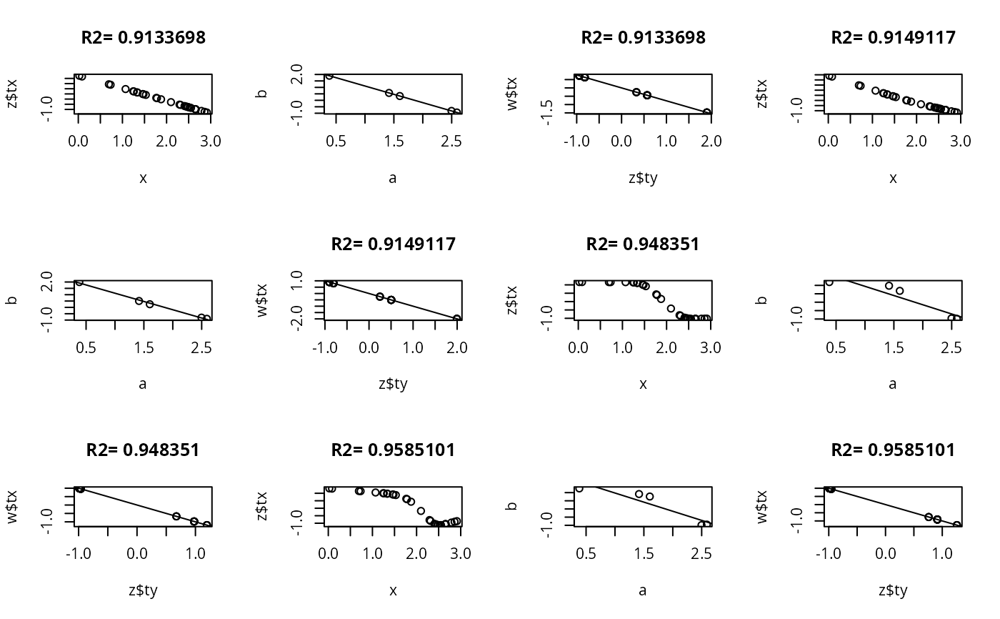
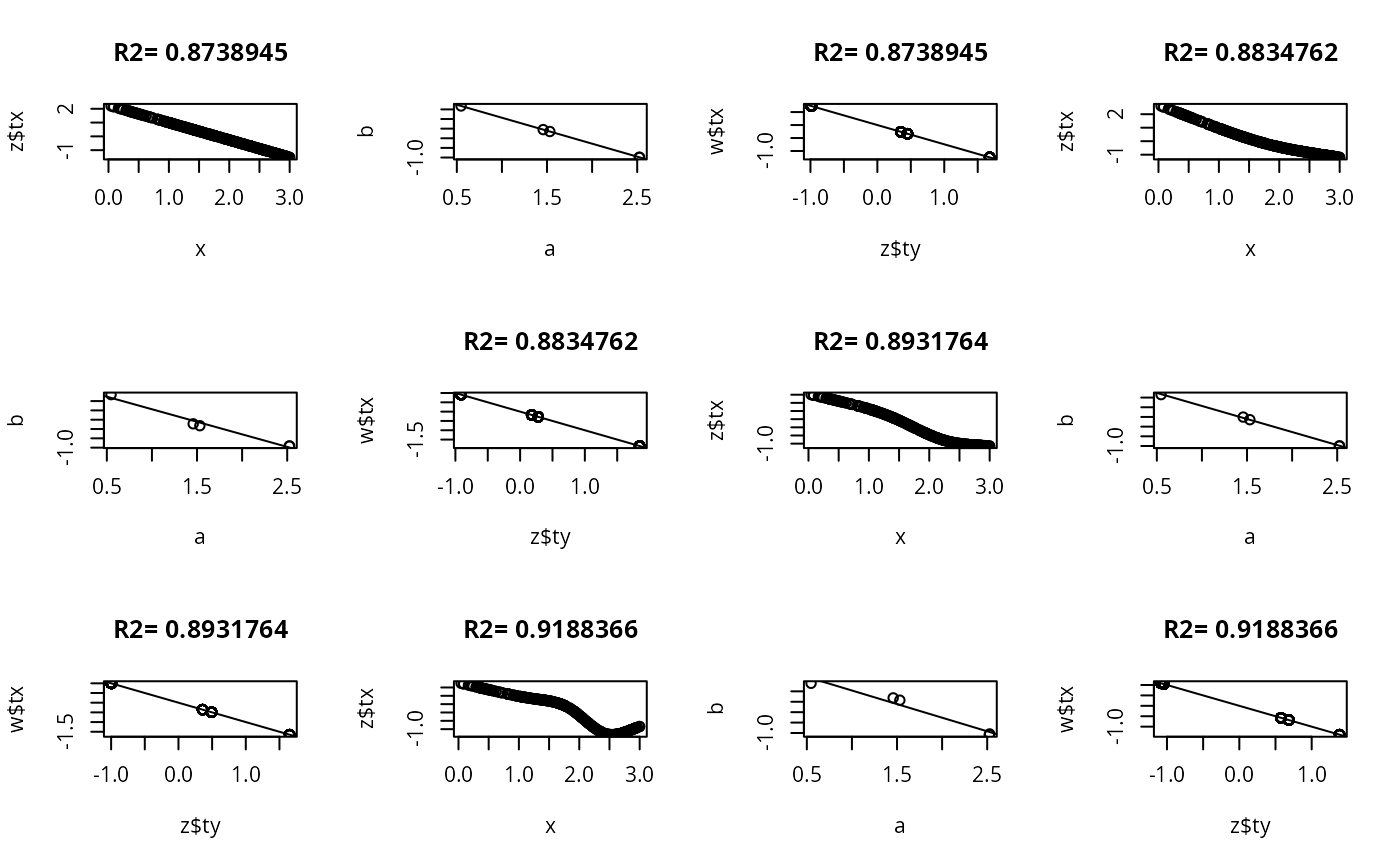
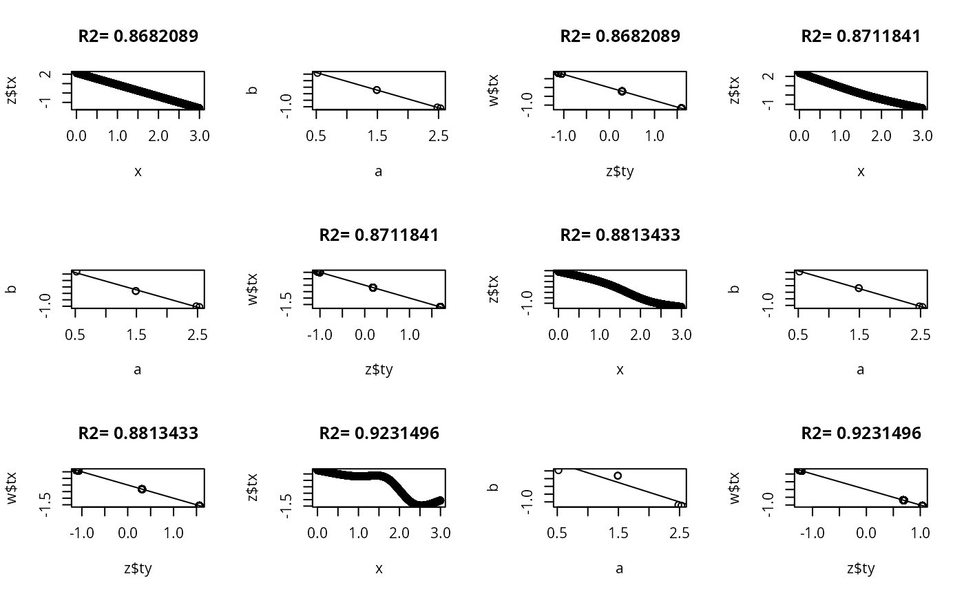
for(n in ns) {
y <- sample(1:5, n, TRUE)
x <- abs(y-3) + runif(n)
par(mfrow=c(3,4))
for(k in c(0,3:5)) {
z <- areg(x, y, ytype='c', nk=k)
plot(x, z$tx)
title(paste('R2=',format(z$rsquared)))
tapply(z$ty, y, range)
a <- tapply(x,y,mean)
b <- tapply(z$ty,y,mean)
plot(a,b)
abline(lsfit(a,b))
# Should get same result to within linear transformation if reverse x and y
w <- areg(y, x, xtype='c', nk=k)
plot(z$ty, w$tx)
title(paste('R2=',format(w$rsquared)))
abline(lsfit(z$ty, w$tx))
}
}
 par(mfrow=c(2,2))
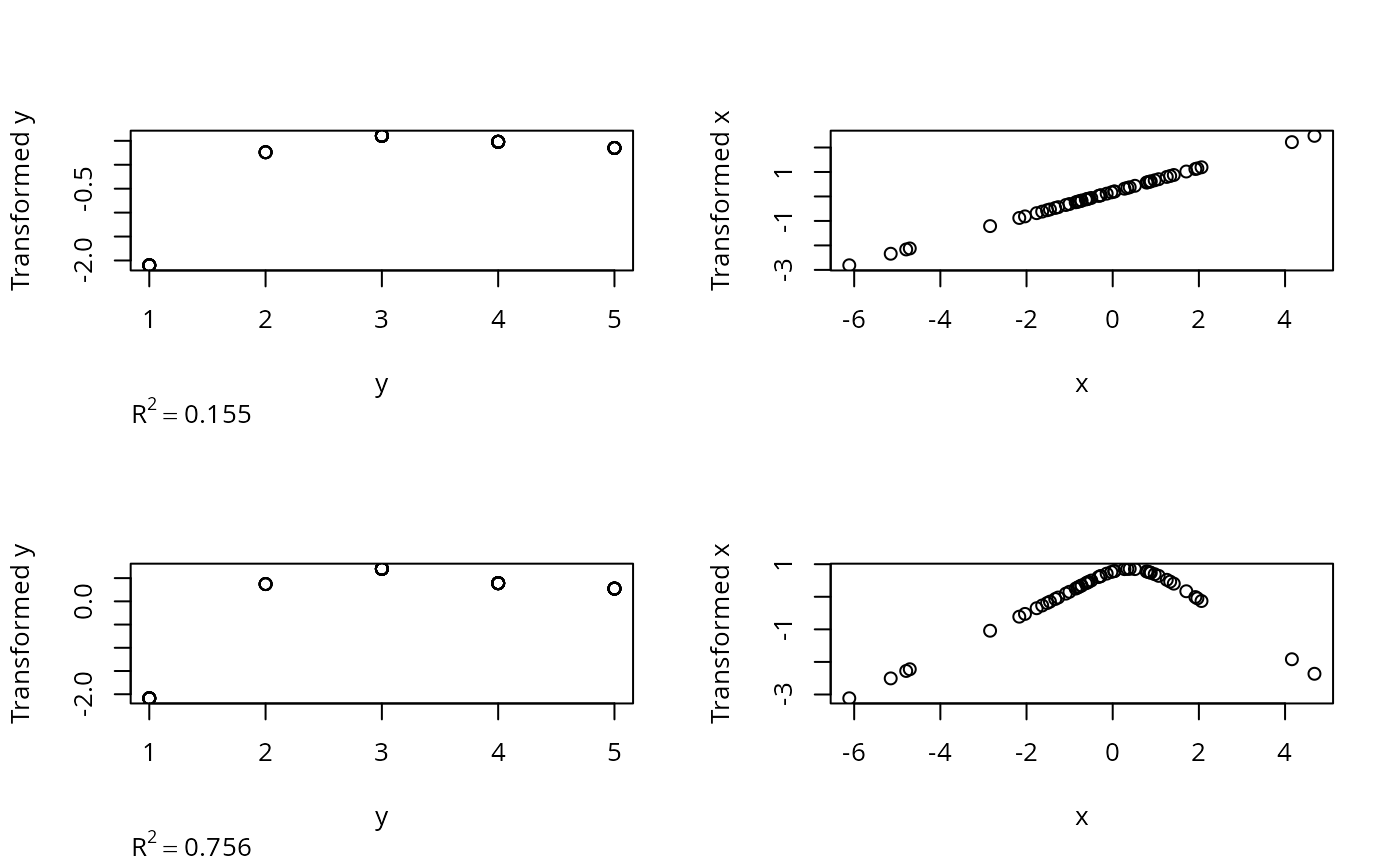
# Example where one category in y differs from others but only in variance of x
n <- 50
y <- sample(1:5,n,TRUE)
x <- rnorm(n)
x[y==1] <- rnorm(sum(y==1), 0, 5)
z <- areg(x,y,xtype='l',ytype='c')
z
#>
#> N: 50 0 observations with NAs deleted.
#> R^2: 0.155 nk: 4 Mean and Median |error|: 2.2, 2
#>
#>
#> type d.f.
#> x l 1
#>
#> y type: c d.f.: 4
#>
plot(z)
z <- areg(x,y,ytype='c')
z
#>
#> N: 50 0 observations with NAs deleted.
#> R^2: 0.756 nk: 4 Mean and Median |error|: 2.2, 2
#>
#>
#> type d.f.
#> x s 3
#>
#> y type: c d.f.: 4
#>
plot(z)
par(mfrow=c(2,2))
# Example where one category in y differs from others but only in variance of x
n <- 50
y <- sample(1:5,n,TRUE)
x <- rnorm(n)
x[y==1] <- rnorm(sum(y==1), 0, 5)
z <- areg(x,y,xtype='l',ytype='c')
z
#>
#> N: 50 0 observations with NAs deleted.
#> R^2: 0.155 nk: 4 Mean and Median |error|: 2.2, 2
#>
#>
#> type d.f.
#> x l 1
#>
#> y type: c d.f.: 4
#>
plot(z)
z <- areg(x,y,ytype='c')
z
#>
#> N: 50 0 observations with NAs deleted.
#> R^2: 0.756 nk: 4 Mean and Median |error|: 2.2, 2
#>
#>
#> type d.f.
#> x s 3
#>
#> y type: c d.f.: 4
#>
plot(z)
 if (FALSE) { # \dontrun{
# Examine overfitting when true transformations are linear
par(mfrow=c(4,3))
for(n in c(200,2000)) {
x <- rnorm(n); y <- rnorm(n) + x
for(nk in c(0,3,5)) {
z <- areg(x, y, nk=nk, crossval=10, B=100)
print(z)
plot(z)
title(paste('n=',n))
}
}
par(mfrow=c(1,1))
# Underfitting when true transformation is quadratic but overfitting
# when y is allowed to be transformed
set.seed(49)
n <- 200
x <- rnorm(n); y <- rnorm(n) + .5*x^2
#areg(x, y, nk=0, crossval=10, B=100)
#areg(x, y, nk=4, ytype='l', crossval=10, B=100)
z <- areg(x, y, nk=4) #, crossval=10, B=100)
z
# Plot x vs. predicted value on original scale. Since y-transform is
# not monotonic, there are multiple y-inverses
xx <- seq(-3.5,3.5,length=1000)
yhat <- predict(z, xx, type='fitted')
plot(x, y, xlim=c(-3.5,3.5))
for(j in 1:ncol(yhat)) lines(xx, yhat[,j], col=j)
# Plot a random sample of possible y inverses
yhats <- predict(z, xx, type='fitted', what='sample')
points(xx, yhats, pch=2)
} # }
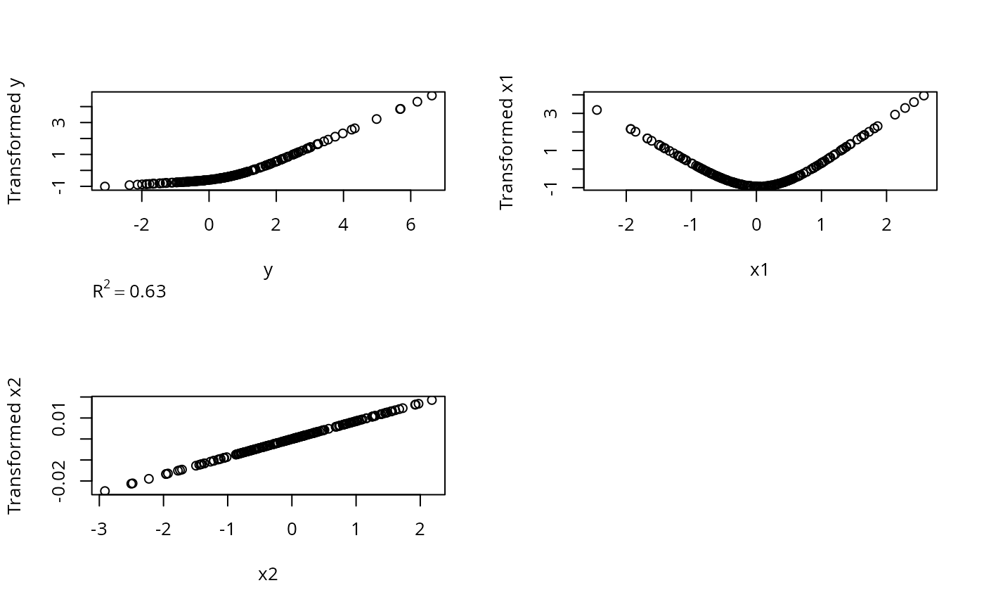
# True transformation of x1 is quadratic, y is linear
n <- 200
x1 <- rnorm(n); x2 <- rnorm(n); y <- rnorm(n) + x1^2
z <- areg(cbind(x1,x2),y,xtype=c('s','l'),nk=3)
par(mfrow=c(2,2))
plot(z)
# y transformation is inverse quadratic but areg gets the same answer by
# making x1 quadratic
n <- 5000
x1 <- rnorm(n); x2 <- rnorm(n); y <- (x1 + rnorm(n))^2
z <- areg(cbind(x1,x2),y,nk=5)
par(mfrow=c(2,2))
if (FALSE) { # \dontrun{
# Examine overfitting when true transformations are linear
par(mfrow=c(4,3))
for(n in c(200,2000)) {
x <- rnorm(n); y <- rnorm(n) + x
for(nk in c(0,3,5)) {
z <- areg(x, y, nk=nk, crossval=10, B=100)
print(z)
plot(z)
title(paste('n=',n))
}
}
par(mfrow=c(1,1))
# Underfitting when true transformation is quadratic but overfitting
# when y is allowed to be transformed
set.seed(49)
n <- 200
x <- rnorm(n); y <- rnorm(n) + .5*x^2
#areg(x, y, nk=0, crossval=10, B=100)
#areg(x, y, nk=4, ytype='l', crossval=10, B=100)
z <- areg(x, y, nk=4) #, crossval=10, B=100)
z
# Plot x vs. predicted value on original scale. Since y-transform is
# not monotonic, there are multiple y-inverses
xx <- seq(-3.5,3.5,length=1000)
yhat <- predict(z, xx, type='fitted')
plot(x, y, xlim=c(-3.5,3.5))
for(j in 1:ncol(yhat)) lines(xx, yhat[,j], col=j)
# Plot a random sample of possible y inverses
yhats <- predict(z, xx, type='fitted', what='sample')
points(xx, yhats, pch=2)
} # }
# True transformation of x1 is quadratic, y is linear
n <- 200
x1 <- rnorm(n); x2 <- rnorm(n); y <- rnorm(n) + x1^2
z <- areg(cbind(x1,x2),y,xtype=c('s','l'),nk=3)
par(mfrow=c(2,2))
plot(z)
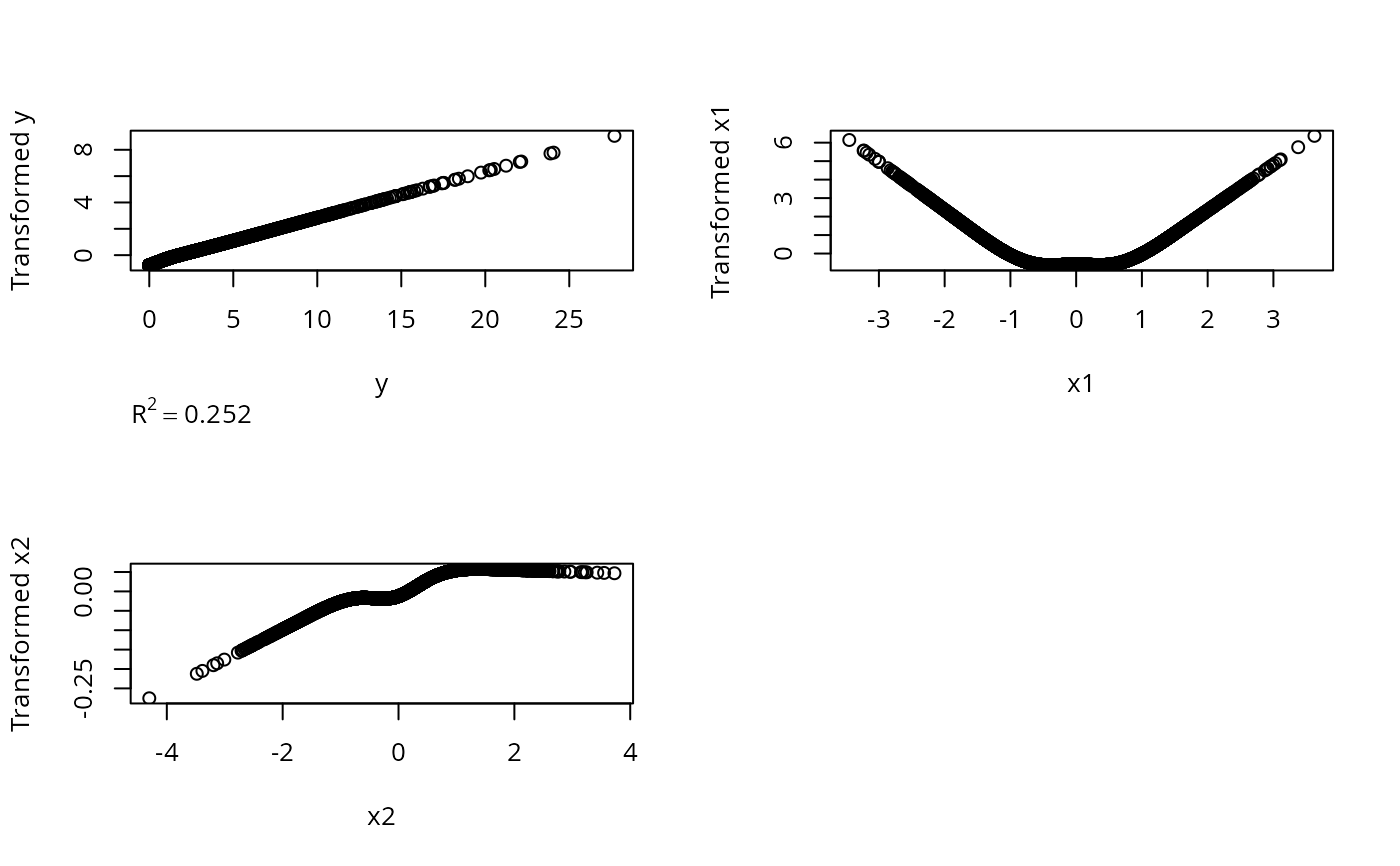
# y transformation is inverse quadratic but areg gets the same answer by
# making x1 quadratic
n <- 5000
x1 <- rnorm(n); x2 <- rnorm(n); y <- (x1 + rnorm(n))^2
z <- areg(cbind(x1,x2),y,nk=5)
par(mfrow=c(2,2))
 plot(z)
# Overfit 20 predictors when no true relationships exist
n <- 1000
x <- matrix(runif(n*20),n,20)
y <- rnorm(n)
z <- areg(x, y, nk=5) # add crossval=4 to expose the problem
# Test predict function
n <- 50
x <- rnorm(n)
y <- rnorm(n) + x
g <- sample(1:3, n, TRUE)
z <- areg(cbind(x,g),y,xtype=c('s','c'))
range(predict(z, cbind(x,g)) - z$linear.predictors)
#> [1] 0 0
plot(z)
# Overfit 20 predictors when no true relationships exist
n <- 1000
x <- matrix(runif(n*20),n,20)
y <- rnorm(n)
z <- areg(x, y, nk=5) # add crossval=4 to expose the problem
# Test predict function
n <- 50
x <- rnorm(n)
y <- rnorm(n) + x
g <- sample(1:3, n, TRUE)
z <- areg(cbind(x,g),y,xtype=c('s','c'))
range(predict(z, cbind(x,g)) - z$linear.predictors)
#> [1] 0 0