Transformations/Imputations using Canonical Variates
transcan.Rdtranscan is a nonlinear additive transformation and imputation
function, and there are several functions for using and operating on
its results. transcan automatically transforms continuous and
categorical variables to have maximum correlation with the best linear
combination of the other variables. There is also an option to use a
substitute criterion - maximum correlation with the first principal
component of the other variables. Continuous variables are expanded
as restricted cubic splines and categorical variables are expanded as
contrasts (e.g., dummy variables). By default, the first canonical
variate is used to find optimum linear combinations of component
columns. This function is similar to ace except that
transformations for continuous variables are fitted using restricted
cubic splines, monotonicity restrictions are not allowed, and
NAs are allowed. When a variable has any NAs,
transformed scores for that variable are imputed using least squares
multiple regression incorporating optimum transformations, or
NAs are optionally set to constants. Shrinkage can be used to
safeguard against overfitting when imputing. Optionally, imputed
values on the original scale are also computed and returned. For this
purpose, recursive partitioning or multinomial logistic models can
optionally be used to impute categorical variables, using what is
predicted to be the most probable category.
By default, transcan imputes NAs with “best
guess” expected values of transformed variables, back transformed to
the original scale. Values thus imputed are most like conditional
medians assuming the transformations make variables' distributions
symmetric (imputed values are similar to conditionl modes for
categorical variables). By instead specifying n.impute,
transcan does approximate multiple imputation from the
distribution of each variable conditional on all other variables.
This is done by sampling n.impute residuals from the
transformed variable, with replacement (a la bootstrapping), or by
default, using Rubin's approximate Bayesian bootstrap, where a sample
of size n with replacement is selected from the residuals on
n non-missing values of the target variable, and then a sample
of size m with replacement is chosen from this sample, where
m is the number of missing values needing imputation for the
current multiple imputation repetition. Neither of these bootstrap
procedures assume normality or even symmetry of residuals. For
sometimes-missing categorical variables, optimal scores are computed
by adding the “best guess” predicted mean score to random
residuals off this score. Then categories having scores closest to
these predicted scores are taken as the random multiple imputations
(impcat = "rpart" is not currently allowed
with n.impute). The literature recommends using n.impute
= 5 or greater. transcan provides only an approximation to
multiple imputation, especially since it “freezes” the
imputation model before drawing the multiple imputations rather than
using different estimates of regression coefficients for each
imputation. For multiple imputation, the aregImpute function
provides a much better approximation to the full Bayesian approach
while still not requiring linearity assumptions.
When you specify n.impute to transcan you can use
fit.mult.impute to re-fit any model n.impute times based
on n.impute completed datasets (if there are any sometimes
missing variables not specified to transcan, some observations
will still be dropped from these fits). After fitting n.impute
models, fit.mult.impute will return the fit object from the
last imputation, with coefficients replaced by the average of
the n.impute coefficient vectors and with a component
var equal to the imputation-corrected variance-covariance
matrix using Rubin's rule. fit.mult.impute can also use the object created by the
mice function in the mice library to draw the
multiple imputations, as well as objects created by
aregImpute. The following components of fit objects are
also replaced with averages over the n.impute model fits:
linear.predictors, fitted.values, stats,
means, icoef, scale, center,
y.imputed.
By specifying fun to fit.mult.impute you can run any
function on the fit objects from completed datasets, with the results
saved in an element named funresults. This facilitates
running bootstrap or cross-validation separately on each completed
dataset and storing all these results in a list for later processing,
e.g., with the rms package processMI function. Note that for
rms-type validation you will need to specify
fitargs=list(x=TRUE,y=TRUE) to fit.mult.impute and to
use special names for fun result components, such as
validate and calibrate so that the result can be
processed with processMI. When simultaneously running multiple
imputation and resampling model validation you may not need values for
n.impute or B (number of bootstraps) as high as usual,
as the total number of repetitions will be n.impute * B.
fit.mult.impute can incorporate robust sandwich variance estimates into
Rubin's rule if robust=TRUE.
For ols models fitted by fit.mult.impute with stacking,
the \(R^2\) measure in the stacked model fit is OK, and
print.ols computes adjusted \(R^2\) using the real sample
size so it is also OK because fit.mult.compute corrects the
stacked error degrees of freedom in the stacked fit object to reflect
the real sample size.
The summary method for transcan prints the function
call, \(R^2\) achieved in transforming each variable, and for each
variable the coefficients of all other transformed variables that are
used to estimate the transformation of the initial variable. If
imputed=TRUE was used in the call to transcan, also uses the
describe function to print a summary of imputed values. If
long = TRUE, also prints all imputed values with observation
identifiers. There is also a simple function print.transcan
which merely prints the transformation matrix and the function call.
It has an optional argument long, which if set to TRUE
causes detailed parameters to be printed. Instead of plotting while
transcan is running, you can plot the final transformations
after the fact using plot.transcan or ggplot.transcan,
if the option trantab = TRUE was specified to transcan.
If in addition the option
imputed = TRUE was specified to transcan,
plot and ggplot will show the location of imputed values
(including multiples) along the axes. For ggplot, imputed
values are shown as red plus signs.
impute method for transcan does imputations for a
selected original data variable, on the original scale (if
imputed=TRUE was given to transcan). If you do not
specify a variable to impute, it will do imputations for all
variables given to transcan which had at least one missing
value. This assumes that the original variables are accessible (i.e.,
they have been attached) and that you want the imputed variables to
have the same names are the original variables. If n.impute was
specified to transcan you must tell impute which
imputation to use. Results are stored in .GlobalEnv
when list.out is not specified (it is recommended to use
list.out=TRUE).
The predict method for transcan computes
predicted variables and imputed values from a matrix of new data.
This matrix should have the same column variables as the original
matrix used with transcan, and in the same order (unless a
formula was used with transcan).
The Function function is a generic function
generator. Function.transcan creates R functions to transform
variables using transformations created by transcan. These
functions are useful for getting predicted values with predictors set
to values on the original scale.
The vcov methods are defined here so that
imputation-corrected variance-covariance matrices are readily
extracted from fit.mult.impute objects, and so that
fit.mult.impute can easily compute traditional covariance
matrices for individual completed datasets.
The subscript method for transcan preserves attributes.
The invertTabulated function does either inverse linear
interpolation or uses sampling to sample qualifying x-values having
y-values near the desired values. The latter is used to get inverse
values having a reasonable distribution (e.g., no floor or ceiling
effects) when the transformation has a flat or nearly flat segment,
resulting in a many-to-one transformation in that region. Sampling
weights are a combination of the frequency of occurrence of x-values
that are within tolInverse times the range of y and the
squared distance between the associated y-values and the target
y-value (aty).
Usage
transcan(x, method=c("canonical","pc"),
         categorical=NULL, asis=NULL, nk, imputed=FALSE, n.impute,
         boot.method=c('approximate bayesian', 'simple'),
         trantab=FALSE, transformed=FALSE,
         impcat=c("score", "multinom", "rpart"),
         mincut=40,
         inverse=c('linearInterp','sample'), tolInverse=.05,
         pr=TRUE, pl=TRUE, allpl=FALSE, show.na=TRUE,
         imputed.actual=c('none','datadensity','hist','qq','ecdf'),
         iter.max=50, eps=.1, curtail=TRUE,
         imp.con=FALSE, shrink=FALSE, init.cat="mode",
         nres=if(boot.method=='simple')200 else 400,
         data, subset, na.action, treeinfo=FALSE,
         rhsImp=c('mean','random'), details.impcat='', ...)

# S3 method for class 'transcan'
summary(object, long=FALSE, digits=6, ...)

# S3 method for class 'transcan'
print(x, long=FALSE, ...)

# S3 method for class 'transcan'
plot(x, ...)

# S3 method for class 'transcan'
ggplot(data, mapping, scale=FALSE, ..., environment)

# S3 method for class 'transcan'
impute(x, var, imputation, name, pos.in, data,
       list.out=FALSE, pr=TRUE, check=TRUE, ...)

fit.mult.impute(formula, fitter, xtrans, data, n.impute, fit.reps=FALSE,
                dtrans, derived, fun, vcovOpts=NULL,
                robust=FALSE, cluster, robmethod=c('huber', 'efron'),
                method=c('ordinary', 'stack', 'only stack'),
                funstack=TRUE, lrt=FALSE,
                pr=TRUE, subset, fitargs)

# S3 method for class 'transcan'
predict(object, newdata, iter.max=50, eps=0.01, curtail=TRUE,
        type=c("transformed","original"),
        inverse, tolInverse, check=FALSE, ...)

Function(object, ...)

# S3 method for class 'transcan'
Function(object, prefix=".", suffix="", pos=-1, ...)

invertTabulated(x, y, freq=rep(1,length(x)),
                aty, name='value',
                inverse=c('linearInterp','sample'),
                tolInverse=0.05, rule=2)

# Default S3 method
vcov(object, regcoef.only=FALSE, ...)

# S3 method for class 'fit.mult.impute'
vcov(object, regcoef.only=TRUE,
                intercepts='mid', ...)
Arguments
- x
a matrix containing continuous variable values and codes for categorical variables. The matrix must have column names (
dimnames). If row names are present, they are used in forming thenamesattribute of imputed values ifimputed = TRUE.xmay also be a formula, in which case the model matrix is created automatically, using data in the calling frame. Advantages of using a formula are thatcategoricalvariables can be determined automatically by a variable being afactorvariable, and variables with two unique levels are modeledasis. Variables with 3 unique values are considered to becategoricalif a formula is specified. For a formula you may also specify that a variable is to remain untransformed by enclosing its name with the identify function, e.g.I(x3). The user may add other variable names to theasisandcategoricalvectors. ForinvertTabulated,xis a vector or a list with three components: the x vector, the corresponding vector of transformed values, and the corresponding vector of frequencies of the pair of original and transformed variables. Forprint,plot,ggplot,impute, andpredict,xis an object created bytranscan.- formula
any R model formula
- fitter
any R,
rms, modeling function (not in quotes) that computes a vector ofcoefficientsand for whichvcovwill return a variance-covariance matrix. E.g.,fitter = lm,glm,ols. At present models involving non-regression parameters (e.g., scale parameters in parametric survival models) are not handled fully.- xtrans
an object created by
transcan,aregImpute, ormice- method
use
method="canonical"or any abbreviation thereof, to use canonical variates (the default).method="pc"transforms a variable instead so as to maximize the correlation with the first principal component of the other variables. Forfit.mult.impute,methodspecifies whether to use standard multiple imputation (the defaultmethod='ordinary') or whether to get final coefficients from stacking all completed datasets and fitting one model. Stacking is required if likelihood ratio tests accounting for imputation are to be done.method='stack'means to do regular MI and stacking, which results in more valid standard errors of coefficient estimates.method='only stack'means that model fits are not done on individual completed datasets, and standard errors will not be very accurate.- categorical
a character vector of names of variables in
xwhich are categorical, for which the ordering of re-scored values is not necessarily preserved. Ifcategoricalis omitted, it is assumed that all variables are continuous (or binary). Setcategorical="*"to treat all variables as categorical.- asis
a character vector of names of variables that are not to be transformed. For these variables, the guts of
lm.fitmethod="qr"is used to impute missing values. You may want to treat binary variablesasis(this is automatic if using a formula). Ifimputed = TRUE, you may want to use "categorical" for binary variables if you want to force imputed values to be one of the original data values. Setasis="*"to treat all variablesasis.- nk
number of knots to use in expanding each continuous variable (not listed in
asis) in a restricted cubic spline function. Default is 3 (yielding 2 parameters for a variable) if \(n < 30\), 4 if \(30 <= n < 100\), and 5 if \(n \ge 100\) (4 parameters).- imputed
Set to
TRUEto return a list containing imputed values on the original scale. If the transformation for a variable is non-monotonic, imputed values are not unique.transcanuses theapproxfunction, which returns the highest value of the variable with the transformed score equalling the imputed score.imputed=TRUEalso causes original-scale imputed values to be shown as tick marks on the top margin of each graph whenshow.na=TRUE(for the final iteration only). For categorical predictors, these imputed values are passed through thejitterfunction so that their frequencies can be visualized. Whenn.imputeis used, eachNAwill haven.imputetick marks.- n.impute
number of multiple imputations. If omitted, single predicted expected value imputation is used.
n.impute=5is frequently recommended.- boot.method
default is to use the approximate Bayesian bootstrap (sample with replacement from sample with replacement of the vector of residuals). You can also specify
boot.method="simple"to use the usual bootstrap one-stage sampling with replacement.- trantab
Set to
TRUEto add an attributetrantabto the returned matrix. This contains a vector of lists each with componentsxandycontaining the unique values and corresponding transformed values for the columns ofx. This is set up to be used easily with theapproxfunction. You must specifytrantab=TRUEif you want to later use thepredict.transcanfunction withtype = "original".- transformed
set to
TRUEto causetranscanto return an objecttransformedcontaining the matrix of transformed variables- impcat
This argument tells how to impute categorical variables on the original scale. The default is
impcat="score"to impute the category whose canonical variate score is closest to the predicted score. Useimpcat="rpart"to impute categorical variables using the values of all other transformed predictors in conjunction with therpartfunction. A better but somewhat slower approach is to useimpcat="multinom"to fit a multinomial logistic model to the categorical variable, at the last iteraction of thetranscanalgorithm. This uses themultinomfunction in the nnet library of the MASS package (which is assumed to have been installed by the user) to fit a polytomous logistic model to the current working transformations of all the other variables (using conditional mean imputation for missing predictors). Multiple imputations are made by drawing multinomial values from the vector of predicted probabilities of category membership for the missing categorical values.- mincut
If
imputed=TRUE, there are categorical variables, andimpcat = "rpart",mincutspecifies the lowest node size that will be allowed to be split. The default is 40.- inverse
By default, imputed values are back-solved on the original scale using inverse linear interpolation on the fitted tabulated transformed values. This will cause distorted distributions of imputed values (e.g., floor and ceiling effects) when the estimated transformation has a flat or nearly flat section. To instead use the
invertTabulatedfunction (see above) with the"sample"option, specifyinverse="sample".- tolInverse
the multiplyer of the range of transformed values, weighted by
freqand by the distance measure, for determining the set of x values having y values within a tolerance of the value ofatyininvertTabulated. Forpredict.transcan,inverseandtolInverseare obtained from options that were specified totranscanby default. Otherwise, if not specified by the user, these default to the defaults used toinvertTabulated.- pr
For
transcan, set toFALSEto suppress printing \(R^2\) and shrinkage factors. Setimpute.transcan=FALSEto suppress messages concerning the number ofNAvalues imputed. Setfit.mult.impute=FALSEto suppress printing variance inflation factors accounting for imputation, rate of missing information, and degrees of freedom.- pl
Set to
FALSEto suppress plotting the final transformations with distribution of scores for imputed values (ifshow.na=TRUE).- allpl
Set to
TRUEto plot transformations for intermediate iterations.- show.na
Set to
FALSEto suppress the distribution of scores assigned to missing values (as tick marks on the right margin of each graph). See alsoimputed.- imputed.actual
The default is "none" to suppress plotting of actual vs. imputed values for all variables having any
NAvalues. Other choices are "datadensity" to usedatadensityto make a single plot, "hist" to make a series of back-to-back histograms, "qq" to make a series of q-q plots, or "ecdf" to make a series of empirical cdfs. Forimputed.actual="datadensity"for example you get a rug plot of the non-missing values for the variable with beneath it a rug plot of the imputed values. Whenimputed.actualis not "none",imputedis automatically set toTRUE.- iter.max
maximum number of iterations to perform for
transcanorpredict. Forpredict, only one iteration is used if there are noNAvalues in the data or ifimp.conwas used.- eps
convergence criterion for
transcanandpredict.epsis the maximum change in transformed values from one iteration to the next. If for a given iteration all new transformations of variables differ by less thaneps(with or without negating the transformation to allow for “flipping”) from the transformations in the previous iteration, one more iteration is done fortranscan. During this last iteration, individual transformations are not updated but coefficients of transformations are. This improves stability of coefficients of canonical variates on the right-hand-side.epsis ignored whenrhsImp="random".- curtail
for
transcan, causes imputed values on the transformed scale to be truncated so that their ranges are within the ranges of non-imputed transformed values. Forpredict,curtaildefaults toTRUEto truncate predicted transformed values to their ranges in the original fit (xt).- imp.con
for
transcan, set toTRUEto imputeNAvalues on the original scales with constants (medians or most frequent category codes). Set to a vector of constants to instead always use these constants for imputation. These imputed values are ignored when fitting the current working transformation for asingle variable.- shrink
default is
FALSEto use ordinary least squares or canonical variate estimates. For the purposes of imputingNAs, you may want to setshrink=TRUEto avoid overfitting when developing a prediction equation to predict each variables from all the others (see details below).- init.cat
method for initializing scorings of categorical variables. Default is "mode" to use a dummy variable set to 1 if the value is the most frequent value (this is the default). Use "random" to use a random 0-1 variable. Set to "asis" to use the original integer codes asstarting scores.
- nres
number of residuals to store if
n.imputeis specified. If the dataset has fewer thannresobservations, all residuals are saved. Otherwise a random sample of the residuals of lengthnreswithout replacement is saved. The default fornresis higher ifboot.method="approximate bayesian".- data
Data frame used to fill the formula. For
ggplotis the result oftranscanwithtrantab=TRUE.- subset
an integer or logical vector specifying the subset of observations to fit
- na.action
These may be used if
xis a formula. The defaultna.actionisna.retain(defined bytranscan) which keeps all observations with anyNAvalues. Forimpute.transcan,datais a data frame to use as the source of variables to be imputed, rather than usingpos.in. Forfit.mult.impute,datais mandatory and is a data frame containing the data to be used in fitting the model but before imputations are applied. Variables omitted fromdataare assumed to be available from frame1 and do not need to be imputed.- treeinfo
Set to
TRUEto get additional information printed whenimpcat="rpart", such as the predicted probabilities of category membership.- rhsImp
Set to "random" to use random draw imputation when a sometimes missing variable is moved to be a predictor of other sometimes missing variables. Default is
rhsImp="mean", which uses conditional mean imputation on the transformed scale. Residuals used are residuals from the transformed scale. When "random" is used,transcanruns 5 iterations and ignoreseps.- details.impcat
set to a character scalar that is the name of a category variable to include in the resulting
transcanobject an elementdetails.impcatcontaining details of how the categorical variable was multiply imputed.- ...
arguments passed to
scat1d. Forggplot.transcan, these arguments are passed tofacet_wrap, e.g.ncol=2.- long
for
summary, set toTRUEto print all imputed values. Forprint, set toTRUEto print details of transformations/imputations.- digits
number of significant digits for printing values by
summary- scale
for
ggplot.transcansetscale=TRUEto scale transformed values to [0,1] before plotting.- mapping,environment
not used; needed because of rules about generics
- var
For
impute, is a variable that was originally a column inx, for which imputated values are to be filled in.imputed=TRUEmust have been used intranscan. Omitvarto impute all variables, creating new variables in positionpos(seeassign).- imputation
specifies which of the multiple imputations to use for filling in
NAvalues- name
name of variable to impute, for
imputefunction. Default is character string version of the second argument (var) in the call toimpute. ForinvertTabulated, is the name of variable being transformed (used only for warning messages).- pos.in
location as defined by
assignto find variables that need to be imputed, when all variables are to be imputed automatically byimpute.transcan(i.e., when no input variable name is specified). Default is position that contains the first variable to be imputed.- list.out
If
varis not specified, you can setlist.out=TRUEto haveimpute.transcanreturn a list containing variables with needed values imputed. This list will contain a single imputation. Variables not needing imputation are copied to the list as-is. You can use this list for analysis just like a data frame.- check
set to
FALSEto suppress certain warning messages- newdata
a new data matrix for which to compute transformed variables. Categorical variables must use the same integer codes as were used in the call to
transcan. If a formula was originally specified totranscan(instead of a data matrix),newdatais optional and if given must be a data frame; a model frame is generated automatically from the previous formula. Thena.actionis handled automatically, and the levels for factor variables must be the same and in the same order as were used in the original variables specified in the formula given totranscan.- fit.reps
set to
TRUEto save all fit objects from the fit for each imputation infit.mult.impute. Then the object returned will have a componentfitswhich is a list whose i'th element is the i'th fit object.- dtrans
provides an approach to creating derived variables from a single filled-in dataset. The function specified as
dtranscan even reshape the imputed dataset. An example of such usage is fitting time-dependent covariates in a Cox model that are created by “start,stop” intervals. Imputations may be done on a one record per subject data frame that is converted bydtransto multiple records per subject. The imputation can enforce consistency of certain variables across records so that for example a missing value of sex will not be imputed as male for one of the subject's records and female as another. An example of howdtransmight be specified isdtrans=function(w) {w$age <- w$years + w$months/12; w}wheremonthsmight havebeen imputed butyearswas never missing. An outline for using `dtrans` to impute missing baseline variables in a longitudinal analysis appears in Details below.- derived
an expression containing R expressions for computing derived variables that are used in the model formula. This is useful when multiple imputations are done for component variables but the actual model uses combinations of these (e.g., ratios or other derivations). For a single derived variable you can specify for example
derived=expression(ratio <- weight/height). For multiple derived variables use the formderived=expression({ratio <- weight/height; product <- weight*height})or put the expression on separate input lines. To monitor the multiply-imputed derived variables you can add to theexpressiona command such asprint(describe(ratio)). See the example below. Note thatderivedis not yet implemented.- fun
a function of a fit made on one of the completed datasets. Typical uses are bootstrap model validations. The result of
funfor imputationiis placed in theith element of a list that is returned in thefit.mult.imputeobject element namedfunresults. See thermsprocessMIfunction for help in processing these results for the cases ofvalidateandcalibrate.- vcovOpts
a list of named additional arguments to pass to the
vcovmethod forfitter. Useful forormmodels for retaining all intercepts (vcovOpts=list(intercepts='all')) instead of just the middle one.- robust
set to
TRUEto havefit.mult.imputecall thermspackagerobcovfunction on each fit on a completed dataset. Whenclusteris given,robustis forced toTRUE.- cluster
a vector of cluster IDs that is the same length of the number of rows in the dataset being analyzed. When specified,
robustis assumed to beTRUE, and thermsrobcovfunction is called with theclustervector given as its second argument.- robmethod
see the
robcovfunction'smethodargument- funstack
set to
FALSEto not runfunon the stacked dataset, making ann.impute+1 element offunresults- lrt
set to
TRUEto havemethod, fun, fitargsset appropriately automatically so thatprocessMIcan be used to get likelihood ratio tests. When doing this,funmay not be specified by the user.- fitargs
a list of extra arguments to pass to
fitter, used especially withfun. Whenrobust=TRUEthe argumentsx=TRUE, y=TRUEare automatically added tofitargs.- type
By default, the matrix of transformed variables is returned, with imputed values on the transformed scale. If you had specified
trantab=TRUEtotranscan, specifyingtype="original"does the table look-ups with linear interpolation to return the input matrixxbut with imputed values on the original scale inserted forNAvalues. For categorical variables, the method used here is to select the category code having a corresponding scaled value closest to the predicted transformed value. This corresponds to the defaultimpcat. Note: imputed values thus returned whentype="original"are single expected value imputations even inn.imputeis given.- object
an object created by
transcan, or an object to be converted to R function code, typically a model fit object of some sort- prefix, suffix
When creating separate R functions for each variable in
x, the name of the new function will beprefixplaced in front of the variable name, andsuffixplaced in back of the name. The default is to use names of the form .varname, where varname is the variable name.- pos
position as in
assignat which to store new functions (forFunction). Default ispos=-1.- y
a vector corresponding to
xforinvertTabulated, if its first argumentxis not a list- freq
a vector of frequencies corresponding to cross-classified
xandyifxis not a list. Default is a vector of ones.- aty
vector of transformed values at which inverses are desired
- rule
see
approx.transcanassumesruleis always 2.- regcoef.only
set to
TRUEto makevcov.defaultdelete positions in the covariance matrix for any non-regression coefficients (e.g., log scale parameter frompsmorsurvreg)- intercepts
this is primarily for
ormobjects. Set to"none"to discard all intercepts from the covariance matrix, or to"all"or"mid"to keep all elements generated byorm(ormonly outputs the covariance matrix for the intercept corresponding to the median). You can also setinterceptsto a vector of subscripts for selecting particular intercepts in a multi-intercept model.
Value
For transcan, a list of class transcan with elements
- call
(with the function call)
- iter
(number of iterations done)
- rsq, rsq.adj
containing the \(R^2\)s and adjusted \(R^2\)s achieved in predicting each variable from all the others
- categorical
the values supplied for
categorical- asis
the values supplied for
asis- coef
the within-variable coefficients used to compute the first canonical variate
- xcoef
the (possibly shrunk) across-variables coefficients of the first canonical variate that predicts each variable in-turn.
- parms
the parameters of the transformation (knots for splines, contrast matrix for categorical variables)
- fillin
the initial estimates for missing values (
NAif variable never missing)- ranges
the matrix of ranges of the transformed variables (min and max in first and secondrow)
- scale
a vector of scales used to determine convergence for a transformation.
- formula
the formula (if
xwas a formula)
, and optionally a vector of shrinkage factors used for predicting
each variable from the others. For asis variables, the scale
is the average absolute difference about the median. For other
variables it is unity, since canonical variables are standardized.
For xcoef, row i has the coefficients to predict
transformed variable i, with the column for the coefficient of
variable i set to NA. If imputed=TRUE was given,
an optional element imputed also appears. This is a list with
the vector of imputed values (on the original scale) for each variable
containing NAs. Matrices rather than vectors are returned if
n.impute is given. If trantab=TRUE, the trantab
element also appears, as described above. If n.impute > 0,
transcan also returns a list residuals that can be used
for future multiple imputation.
impute returns a vector (the same length as var) of
class impute with NA values imputed.
predict returns a matrix with the same number of columns or
variables as were in x.
fit.mult.impute returns a fit object that is a modification of
the fit object created by fitting the completed dataset for the final
imputation. The var matrix in the fit object has the
imputation-corrected variance-covariance matrix. coefficients
is the average (over imputations) of the coefficient vectors,
variance.inflation.impute is a vector containing the ratios of
the diagonals of the between-imputation variance matrix to the
diagonals of the average apparent (within-imputation) variance
matrix. missingInfo is
Rubin's rate of missing information and dfmi is
Rubin's degrees of freedom for a t-statistic
for testing a single parameter. The last two objects are vectors
corresponding to the diagonal of the variance matrix. The class
"fit.mult.impute" is prepended to the other classes produced by
the fitting function.
When method is not 'ordinary', i.e., stacking is used,
fit.mult.impute returns a modified fit object that is computed
on all completed datasets combined, with most all statistics that are
functions of the sample size corrected to the real sample size.
Elements in the fit such as residuals will have length equal to
the real sample size times the number of imputations.
fit.mult.impute stores intercepts attributes in the
coefficient matrix and in var for orm fits.
Details
The starting approximation to the transformation for each variable is
taken to be the original coding of the variable. The initial
approximation for each missing value is taken to be the median of the
non-missing values for the variable (for continuous ones) or the most
frequent category (for categorical ones). Instead, if imp.con
is a vector, its values are used for imputing NA values. When
using each variable as a dependent variable, NA values on that
variable cause all observations to be temporarily deleted. Once a new
working transformation is found for the variable, along with a model
to predict that transformation from all the other variables, that
latter model is used to impute NA values in the selected
dependent variable if imp.con is not specified.
When that variable is used to predict a new dependent variable, the
current working imputed values are inserted. Transformations are
updated after each variable becomes a dependent variable, so the order
of variables on x could conceivably make a difference in the
final estimates. For obtaining out-of-sample
predictions/transformations, predict uses the same
iterative procedure as transcan for imputation, with the same
starting values for fill-ins as were used by transcan. It also
(by default) uses a conservative approach of curtailing transformed
variables to be within the range of the original ones. Even when
method = "pc" is specified, canonical variables are used for
imputing missing values.
Note that fitted transformations, when evaluated at imputed variable
values (on the original scale), will not precisely match the
transformed imputed values returned in xt. This is because
transcan uses an approximate method based on linear
interpolation to back-solve for imputed values on the original scale.
Shrinkage uses the method of
Van Houwelingen and Le Cessie (1990) (similar to
Copas, 1983). The shrinkage factor is
$$\frac{1-\frac{(1-R2)(n-1)}{n-k-1}}{R2}$$
where R2 is the apparent \(R^2\)d for predicting the
variable, n is the number of non-missing values, and k is
the effective number of degrees of freedom (aside from intercepts). A
heuristic estimate is used for k:
A - 1 + sum(max(0,Bi - 1))/m + m, where
A is the number of d.f. required to represent the variable being
predicted, the Bi are the number of columns required to
represent all the other variables, and m is the number of all
other variables. Division by m is done because the
transformations for the other variables are fixed at their current
transformations the last time they were being predicted. The
\(+ m\) term comes from the number of coefficients estimated
on the right hand side, whether by least squares or canonical
variates. If a shrinkage factor is negative, it is set to 0. The
shrinkage factor is the ratio of the adjusted \(R^2\)d to
the ordinary \(R^2\)d. The adjusted \(R^2\)d is
$$1-\frac{(1-R2)(n-1)}{n-k-1}$$
which is also set to zero if it is negative. If shrink=FALSE
and the adjusted \(R^2\)s are much smaller than the
ordinary \(R^2\)s, you may want to run transcan
with shrink=TRUE.
Canonical variates are scaled to have variance of 1.0, by multiplying
canonical coefficients from cancor by
\(\sqrt{n-1}\).
When specifying a non-rms library fitting function to
fit.mult.impute (e.g., lm, glm),
running the result of fit.mult.impute through that fit's
summary method will not use the imputation-adjusted
variances. You may obtain the new variances using fit$var or
vcov(fit).
When you specify a rms function to fit.mult.impute (e.g.
lrm, ols, cph,
psm, bj, Rq,
Gls, Glm), automatically computed
transformation parameters (e.g., knot locations for
rcs) that are estimated for the first imputation are
used for all other imputations. This ensures that knot locations will
not vary, which would change the meaning of the regression
coefficients.
Warning: even though fit.mult.impute takes imputation into
account when estimating variances of regression coefficient, it does
not take into account the variation that results from estimation of
the shapes and regression coefficients of the customized imputation
equations. Specifying shrink=TRUE solves a small part of this
problem. To fully account for all sources of variation you should
consider putting the transcan invocation inside a bootstrap or
loop, if execution time allows. Better still, use
aregImpute or a package such as as mice that uses
real Bayesian posterior realizations to multiply impute missing values
correctly.
It is strongly recommended that you use the Hmisc naclus
function to determine is there is a good basis for imputation.
naclus will tell you, for example, if systolic blood
pressure is missing whenever diastolic blood pressure is missing. If
the only variable that is well correlated with diastolic bp is
systolic bp, there is no basis for imputing diastolic bp in this case.
At present, predict does not work with multiple imputation.
When calling fit.mult.impute with glm as the
fitter argument, if you need to pass a family argument
to glm do it by quoting the family, e.g.,
family="binomial".
fit.mult.impute will not work with proportional odds models
when regression imputation was used (as opposed to predictive mean
matching). That's because regression imputation will create values of
the response variable that did not exist in the dataset, altering the
intercept terms in the model.
You should be able to use a variable in the formula given to
fit.mult.impute as a numeric variable in the regression model
even though it was a factor variable in the invocation of
transcan. Use for example fit.mult.impute(y ~ codes(x),
lrm, trans) (thanks to Trevor Thompson
trevor@hp5.eushc.org).
Here is an outline of the steps necessary to impute baseline variables
using the dtrans argument, when the analysis to be repeated by
fit.mult.impute is a longitudinal analysis (using
e.g. Gls).
Create a one row per subject data frame containing baseline variables plus follow-up variables that are assigned to windows. For example, you may have dozens of repeated measurements over years but you capture the measurements at the times measured closest to 1, 2, and 3 years after study entry
Make sure the dataset contains the subject ID
This dataset becomes the one passed to
aregImputeasdata=. You will be imputing missing baseline variables from follow-up measurements defined at fixed times.Have another dataset with all the non-missing follow-up values on it, one record per measurement time per subject. This dataset should not have the baseline variables on it, and the follow-up measurements should not be named the same as the baseline variable(s); the subject ID must also appear
Add the dtrans argument to
fit.mult.imputeto define a function with one argument representing the one record per subject dataset with missing values filled it from the current imputation. This function merges the above 2 datasets; the returned value of this function is the merged data frame.This merged-on-the-fly dataset is the one handed by
fit.mult.imputeto your fitting function, so variable names in the formula given tofit.mult.imputemust matched the names created by the merge
Author
Frank Harrell
Department of Biostatistics
Vanderbilt University
fh@fharrell.com
References
Kuhfeld, Warren F: The PRINQUAL Procedure. SAS/STAT User's Guide, Fourth Edition, Volume 2, pp. 1265–1323, 1990.
Van Houwelingen JC, Le Cessie S: Predictive value of statistical models. Statistics in Medicine 8:1303–1325, 1990.
Copas JB: Regression, prediction and shrinkage. JRSS B 45:311–354, 1983.
He X, Shen L: Linear regression after spline transformation. Biometrika 84:474–481, 1997.
Little RJA, Rubin DB: Statistical Analysis with Missing Data. New York: Wiley, 1987.
Rubin DJ, Schenker N: Multiple imputation in health-care databases: An overview and some applications. Stat in Med 10:585–598, 1991.
Faris PD, Ghali WA, et al:Multiple imputation versus data enhancement for dealing with missing data in observational health care outcome analyses. J Clin Epidem 55:184–191, 2002.
See also
aregImpute, impute, naclus,
naplot, ace,
avas, cancor,
prcomp, rcspline.eval,
lsfit, approx, datadensity,
mice, ggplot,
processMI
Examples
if (FALSE) { # \dontrun{
x <- cbind(age, disease, blood.pressure, pH)
#cbind will convert factor object `disease' to integer
par(mfrow=c(2,2))
x.trans <- transcan(x, categorical="disease", asis="pH",
transformed=TRUE, imputed=TRUE)
summary(x.trans) #Summary distribution of imputed values, and R-squares
f <- lm(y ~ x.trans$transformed) #use transformed values in a regression
#Now replace NAs in original variables with imputed values, if not
#using transformations
age <- impute(x.trans, age)
disease <- impute(x.trans, disease)
blood.pressure <- impute(x.trans, blood.pressure)
pH <- impute(x.trans, pH)
#Do impute(x.trans) to impute all variables, storing new variables under
#the old names
summary(pH) #uses summary.impute to tell about imputations
#and summary.default to tell about pH overall
# Get transformed and imputed values on some new data frame xnew
newx.trans <- predict(x.trans, xnew)
w <- predict(x.trans, xnew, type="original")
age <- w[,"age"] #inserts imputed values
blood.pressure <- w[,"blood.pressure"]
Function(x.trans) #creates .age, .disease, .blood.pressure, .pH()
#Repeat first fit using a formula
x.trans <- transcan(~ age + disease + blood.pressure + I(pH),
imputed=TRUE)
age <- impute(x.trans, age)
predict(x.trans, expand.grid(age=50, disease="pneumonia",
blood.pressure=60:260, pH=7.4))
z <- transcan(~ age + factor(disease.code), # disease.code categorical
transformed=TRUE, trantab=TRUE, imputed=TRUE, pl=FALSE)
ggplot(z, scale=TRUE)
plot(z$transformed)
} # }
# Multiple imputation and estimation of variances and covariances of
# regression coefficient estimates accounting for imputation
set.seed(1)
x1 <- factor(sample(c('a','b','c'),100,TRUE))
x2 <- (x1=='b') + 3*(x1=='c') + rnorm(100)
y <- x2 + 1*(x1=='c') + rnorm(100)
x1[1:20] <- NA
x2[18:23] <- NA
d <- data.frame(x1,x2,y)
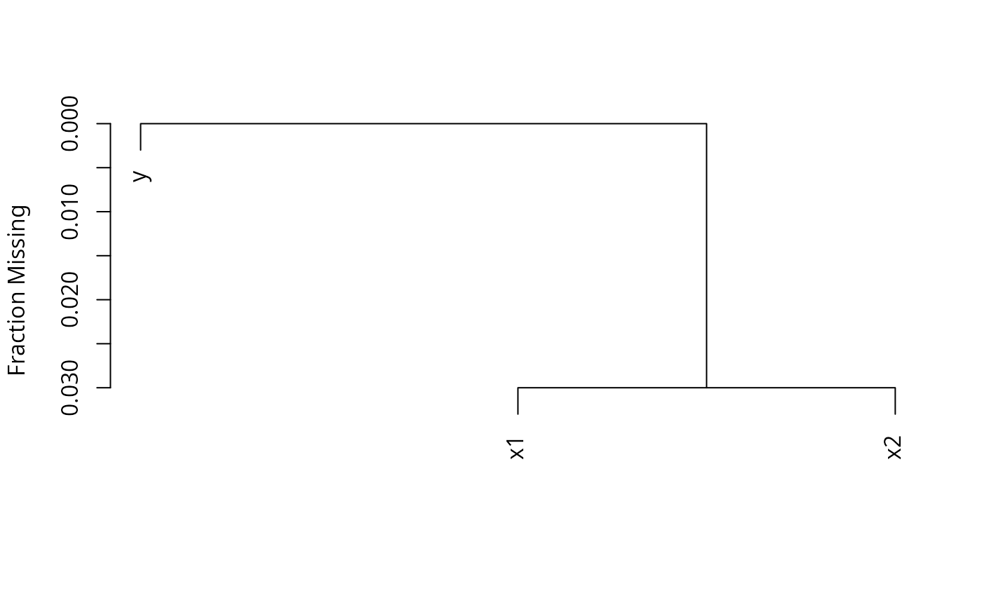
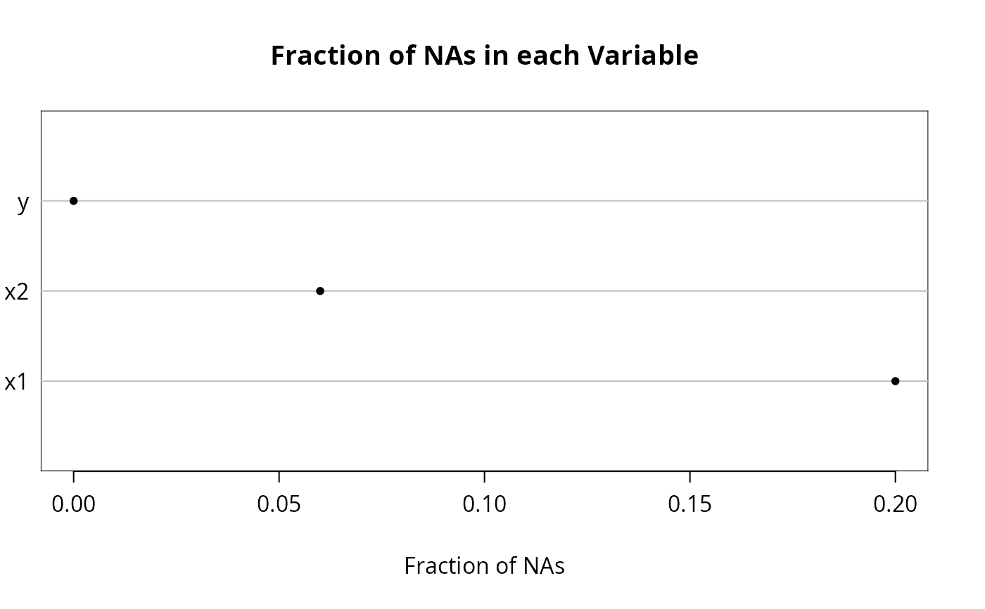
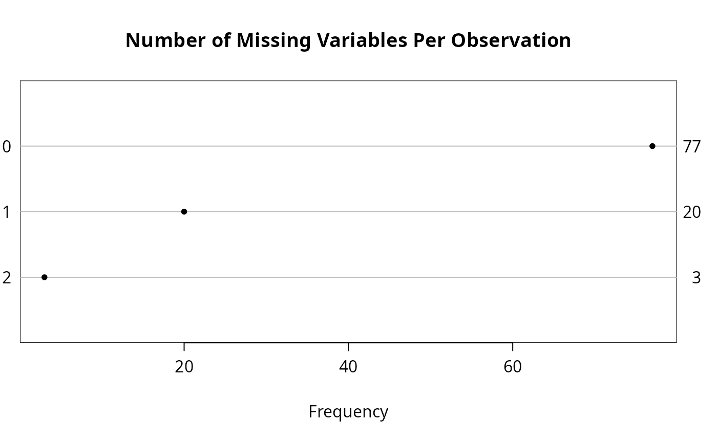
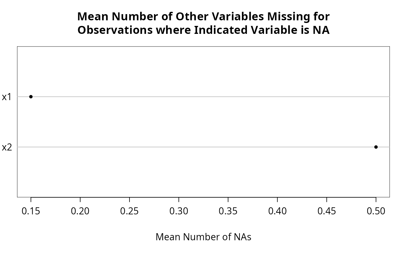
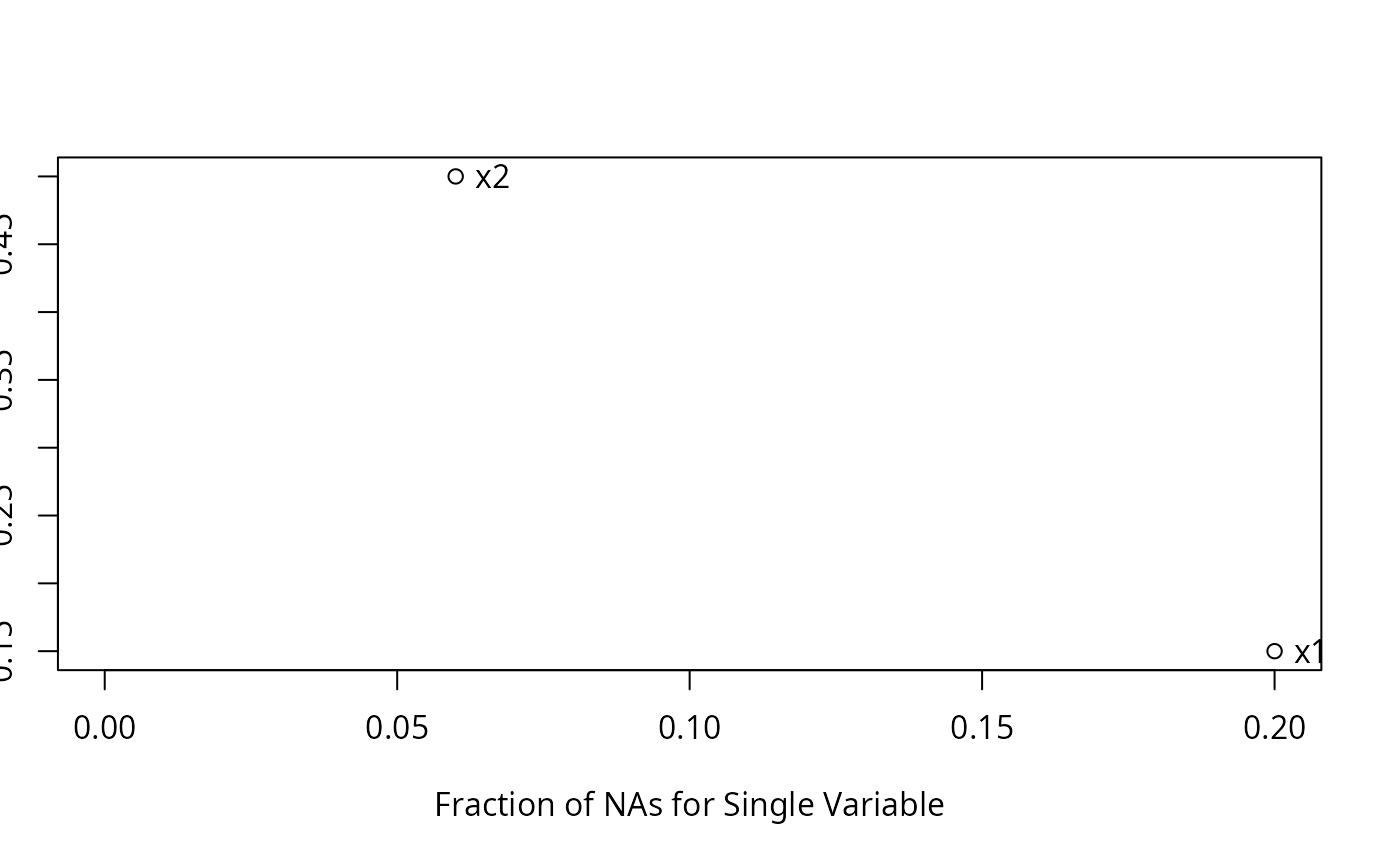
n <- naclus(d)
plot(n); naplot(n) # Show patterns of NAs
 f <- transcan(~y + x1 + x2, n.impute=10, shrink=FALSE, data=d)
#> Warning: transcan provides only an approximation to true multiple imputation.
#> A better approximation is provided by the aregImpute function.
#> The MICE and other S libraries provide imputations from Bayesian posterior distributions.
#> Convergence criterion:0.666 0.173 0.068
f <- transcan(~y + x1 + x2, n.impute=10, shrink=FALSE, data=d)
#> Warning: transcan provides only an approximation to true multiple imputation.
#> A better approximation is provided by the aregImpute function.
#> The MICE and other S libraries provide imputations from Bayesian posterior distributions.
#> Convergence criterion:0.666 0.173 0.068


 #> 0.022
#> Convergence in 5 iterations
#> R-squared achieved in predicting each variable:
#>
#> y x1 x2
#> 0.838 0.748 0.815
#>
#> Adjusted R-squared:
#>
#> y x1 x2
#> 0.826 0.727 0.800
options(digits=3)
summary(f)
#> transcan(x = ~y + x1 + x2, n.impute = 10, shrink = FALSE, data = d)
#>
#> Iterations: 5
#>
#> R-squared achieved in predicting each variable:
#>
#> y x1 x2
#> 0.838 0.748 0.815
#>
#> Adjusted R-squared:
#>
#> y x1 x2
#> 0.826 0.727 0.800
#>
#> Coefficients of canonical variates for predicting each (row) variable
#>
#> y x1 x2
#> y -0.39 0.58
#> x1 -0.65 -0.49
#> x2 0.67 -0.35
#>
#> Summary of imputed values
#>
#> x1
#> n missing distinct Info Mean pMedian Gmd
#> 200 0 3 0.803 1.75 2 0.9196
#>
#> Value 1 2 3
#> Frequency 110 30 60
#> Proportion 0.55 0.15 0.30
#> x2
#> n missing distinct Info Mean pMedian Gmd .05
#> 60 0 53 0.999 1.128 1.116 1.922 -1.4251
#> .10 .25 .50 .75 .90 .95
#> -0.8569 -0.3847 1.0902 2.5492 3.2485 3.7237
#>
#> lowest : -1.4251 -1.04073 -0.83646 -0.784439 -0.711954
#> highest: 3.48258 3.70141 4.1473 4.58272 4.82811
#>
#> Starting estimates for imputed values:
#>
#> y x1 x2
#> 1.33 2.00 1.26
f <- transcan(~y + x1 + x2, n.impute=10, shrink=TRUE, data=d)
#> Warning: transcan provides only an approximation to true multiple imputation.
#> A better approximation is provided by the aregImpute function.
#> The MICE and other S libraries provide imputations from Bayesian posterior distributions.
#> Convergence criterion:0.654 0.14 0.059
#> 0.022
#> Convergence in 5 iterations
#> R-squared achieved in predicting each variable:
#>
#> y x1 x2
#> 0.838 0.748 0.815
#>
#> Adjusted R-squared:
#>
#> y x1 x2
#> 0.826 0.727 0.800
options(digits=3)
summary(f)
#> transcan(x = ~y + x1 + x2, n.impute = 10, shrink = FALSE, data = d)
#>
#> Iterations: 5
#>
#> R-squared achieved in predicting each variable:
#>
#> y x1 x2
#> 0.838 0.748 0.815
#>
#> Adjusted R-squared:
#>
#> y x1 x2
#> 0.826 0.727 0.800
#>
#> Coefficients of canonical variates for predicting each (row) variable
#>
#> y x1 x2
#> y -0.39 0.58
#> x1 -0.65 -0.49
#> x2 0.67 -0.35
#>
#> Summary of imputed values
#>
#> x1
#> n missing distinct Info Mean pMedian Gmd
#> 200 0 3 0.803 1.75 2 0.9196
#>
#> Value 1 2 3
#> Frequency 110 30 60
#> Proportion 0.55 0.15 0.30
#> x2
#> n missing distinct Info Mean pMedian Gmd .05
#> 60 0 53 0.999 1.128 1.116 1.922 -1.4251
#> .10 .25 .50 .75 .90 .95
#> -0.8569 -0.3847 1.0902 2.5492 3.2485 3.7237
#>
#> lowest : -1.4251 -1.04073 -0.83646 -0.784439 -0.711954
#> highest: 3.48258 3.70141 4.1473 4.58272 4.82811
#>
#> Starting estimates for imputed values:
#>
#> y x1 x2
#> 1.33 2.00 1.26
f <- transcan(~y + x1 + x2, n.impute=10, shrink=TRUE, data=d)
#> Warning: transcan provides only an approximation to true multiple imputation.
#> A better approximation is provided by the aregImpute function.
#> The MICE and other S libraries provide imputations from Bayesian posterior distributions.
#> Convergence criterion:0.654 0.14 0.059
 #> 0.018
#> Convergence in 5 iterations
#> R-squared achieved in predicting each variable:
#>
#> y x1 x2
#> 0.839 0.746 0.815
#>
#> Adjusted R-squared:
#>
#> y x1 x2
#> 0.826 0.726 0.800
#>
#> Shrinkage factors:
#>
#> y x1 x2
#> 0.943 0.951 0.942
summary(f)
#> transcan(x = ~y + x1 + x2, n.impute = 10, shrink = TRUE, data = d)
#>
#> Iterations: 5
#>
#> R-squared achieved in predicting each variable:
#>
#> y x1 x2
#> 0.839 0.746 0.815
#>
#> Adjusted R-squared:
#>
#> y x1 x2
#> 0.826 0.726 0.800
#>
#> Shrinkage factors:
#>
#> y x1 x2
#> 0.943 0.951 0.942
#>
#> Coefficients of canonical variates for predicting each (row) variable
#>
#> y x1 x2
#> y -0.37 0.55
#> x1 -0.62 -0.46
#> x2 0.64 -0.33
#>
#> Summary of imputed values
#>
#> x1
#> n missing distinct Info Mean pMedian Gmd
#> 200 0 3 0.84 1.8 2 0.9246
#>
#> Value 1 2 3
#> Frequency 100 40 60
#> Proportion 0.5 0.2 0.3
#> x2
#> n missing distinct Info Mean pMedian Gmd .05
#> 60 0 53 0.999 1.073 1.081 1.985 -1.425
#> .10 .25 .50 .75 .90 .95
#> -1.357 -0.410 1.235 2.660 3.032 3.508
#>
#> lowest : -1.4251 -1.34996 -1.32854 -0.75174 -0.733979
#> highest: 3.19984 3.48771 3.8897 4.4897 4.98724
#>
#> Starting estimates for imputed values:
#>
#> y x1 x2
#> 1.33 2.00 1.26
h <- fit.mult.impute(y ~ x1 + x2, lm, f, data=d)
#> Warning: If you use print, summary, or anova on the result, lm methods use the
#> sum of squared residuals rather than the Rubin formula for computing
#> residual variance and standard errors. It is suggested to use ols
#> instead of lm.
#>
#> Wald Statistic Information
#>
#> Variance Inflation Factors Due to Imputation:
#>
#> (Intercept) x1b x1c x2
#> 1.07 1.02 1.03 1.09
#>
#> Fraction of Missing Information:
#>
#> (Intercept) x1b x1c x2
#> 0.06 0.02 0.03 0.09
#>
#> d.f. for t-distribution for Tests of Single Coefficients:
#>
#> (Intercept) x1b x1c x2
#> 2350 21248 9601 1200
#>
#> The following fit components were averaged over the 10 model fits:
#>
#> fitted.values
#>
# Add ,fit.reps=TRUE to save all fit objects in h, then do something like:
# for(i in 1:length(h$fits)) print(summary(h$fits[[i]]))
diag(vcov(h))
#> (Intercept) x1b x1c x2
#> 0.0319 0.0792 0.2020 0.0146
h.complete <- lm(y ~ x1 + x2, na.action=na.omit)
h.complete
#>
#> Call:
#> lm(formula = y ~ x1 + x2, na.action = na.omit)
#>
#> Coefficients:
#> (Intercept) x1b x1c x2
#> 0.0691 0.1052 1.3126 0.9245
#>
diag(vcov(h.complete))
#> (Intercept) x1b x1c x2
#> 0.0467 0.0989 0.2346 0.0153
# Note: had the rms ols function been used in place of lm, any
# function run on h (anova, summary, etc.) would have automatically
# used imputation-corrected variances and covariances
# Example demonstrating how using the multinomial logistic model
# to impute a categorical variable results in a frequency
# distribution of imputed values that matches the distribution
# of non-missing values of the categorical variable
if (FALSE) { # \dontrun{
set.seed(11)
x1 <- factor(sample(letters[1:4], 1000,TRUE))
x1[1:200] <- NA
table(x1)/sum(table(x1))
x2 <- runif(1000)
z <- transcan(~ x1 + I(x2), n.impute=20, impcat='multinom')
table(z$imputed$x1)/sum(table(z$imputed$x1))
# Here is how to create a completed dataset
d <- data.frame(x1, x2)
z <- transcan(~x1 + I(x2), n.impute=5, data=d)
imputed <- impute(z, imputation=1, data=d,
list.out=TRUE, pr=FALSE, check=FALSE)
sapply(imputed, function(x)sum(is.imputed(x)))
sapply(imputed, function(x)sum(is.na(x)))
} # }
# Do single imputation and create a filled-in data frame
z <- transcan(~x1 + I(x2), data=d, imputed=TRUE)
#> Convergence criterion:0.026
#> 0.018
#> Convergence in 5 iterations
#> R-squared achieved in predicting each variable:
#>
#> y x1 x2
#> 0.839 0.746 0.815
#>
#> Adjusted R-squared:
#>
#> y x1 x2
#> 0.826 0.726 0.800
#>
#> Shrinkage factors:
#>
#> y x1 x2
#> 0.943 0.951 0.942
summary(f)
#> transcan(x = ~y + x1 + x2, n.impute = 10, shrink = TRUE, data = d)
#>
#> Iterations: 5
#>
#> R-squared achieved in predicting each variable:
#>
#> y x1 x2
#> 0.839 0.746 0.815
#>
#> Adjusted R-squared:
#>
#> y x1 x2
#> 0.826 0.726 0.800
#>
#> Shrinkage factors:
#>
#> y x1 x2
#> 0.943 0.951 0.942
#>
#> Coefficients of canonical variates for predicting each (row) variable
#>
#> y x1 x2
#> y -0.37 0.55
#> x1 -0.62 -0.46
#> x2 0.64 -0.33
#>
#> Summary of imputed values
#>
#> x1
#> n missing distinct Info Mean pMedian Gmd
#> 200 0 3 0.84 1.8 2 0.9246
#>
#> Value 1 2 3
#> Frequency 100 40 60
#> Proportion 0.5 0.2 0.3
#> x2
#> n missing distinct Info Mean pMedian Gmd .05
#> 60 0 53 0.999 1.073 1.081 1.985 -1.425
#> .10 .25 .50 .75 .90 .95
#> -1.357 -0.410 1.235 2.660 3.032 3.508
#>
#> lowest : -1.4251 -1.34996 -1.32854 -0.75174 -0.733979
#> highest: 3.19984 3.48771 3.8897 4.4897 4.98724
#>
#> Starting estimates for imputed values:
#>
#> y x1 x2
#> 1.33 2.00 1.26
h <- fit.mult.impute(y ~ x1 + x2, lm, f, data=d)
#> Warning: If you use print, summary, or anova on the result, lm methods use the
#> sum of squared residuals rather than the Rubin formula for computing
#> residual variance and standard errors. It is suggested to use ols
#> instead of lm.
#>
#> Wald Statistic Information
#>
#> Variance Inflation Factors Due to Imputation:
#>
#> (Intercept) x1b x1c x2
#> 1.07 1.02 1.03 1.09
#>
#> Fraction of Missing Information:
#>
#> (Intercept) x1b x1c x2
#> 0.06 0.02 0.03 0.09
#>
#> d.f. for t-distribution for Tests of Single Coefficients:
#>
#> (Intercept) x1b x1c x2
#> 2350 21248 9601 1200
#>
#> The following fit components were averaged over the 10 model fits:
#>
#> fitted.values
#>
# Add ,fit.reps=TRUE to save all fit objects in h, then do something like:
# for(i in 1:length(h$fits)) print(summary(h$fits[[i]]))
diag(vcov(h))
#> (Intercept) x1b x1c x2
#> 0.0319 0.0792 0.2020 0.0146
h.complete <- lm(y ~ x1 + x2, na.action=na.omit)
h.complete
#>
#> Call:
#> lm(formula = y ~ x1 + x2, na.action = na.omit)
#>
#> Coefficients:
#> (Intercept) x1b x1c x2
#> 0.0691 0.1052 1.3126 0.9245
#>
diag(vcov(h.complete))
#> (Intercept) x1b x1c x2
#> 0.0467 0.0989 0.2346 0.0153
# Note: had the rms ols function been used in place of lm, any
# function run on h (anova, summary, etc.) would have automatically
# used imputation-corrected variances and covariances
# Example demonstrating how using the multinomial logistic model
# to impute a categorical variable results in a frequency
# distribution of imputed values that matches the distribution
# of non-missing values of the categorical variable
if (FALSE) { # \dontrun{
set.seed(11)
x1 <- factor(sample(letters[1:4], 1000,TRUE))
x1[1:200] <- NA
table(x1)/sum(table(x1))
x2 <- runif(1000)
z <- transcan(~ x1 + I(x2), n.impute=20, impcat='multinom')
table(z$imputed$x1)/sum(table(z$imputed$x1))
# Here is how to create a completed dataset
d <- data.frame(x1, x2)
z <- transcan(~x1 + I(x2), n.impute=5, data=d)
imputed <- impute(z, imputation=1, data=d,
list.out=TRUE, pr=FALSE, check=FALSE)
sapply(imputed, function(x)sum(is.imputed(x)))
sapply(imputed, function(x)sum(is.na(x)))
} # }
# Do single imputation and create a filled-in data frame
z <- transcan(~x1 + I(x2), data=d, imputed=TRUE)
#> Convergence criterion:0.026
 #> 0.008
#> Convergence in 3 iterations
#> R-squared achieved in predicting each variable:
#>
#> x1 x2
#> 0.618 0.658
#>
#> Adjusted R-squared:
#>
#> x1 x2
#> 0.608 0.650
imputed <- as.data.frame(impute(z, data=d, list.out=TRUE))
#>
#>
#> Imputed missing values with the following frequencies
#> and stored them in variables with their original names:
#>
#> x1 x2
#> 20 6
# Example where multiple imputations are for basic variables and
# modeling is done on variables derived from these
set.seed(137)
n <- 400
x1 <- runif(n)
x2 <- runif(n)
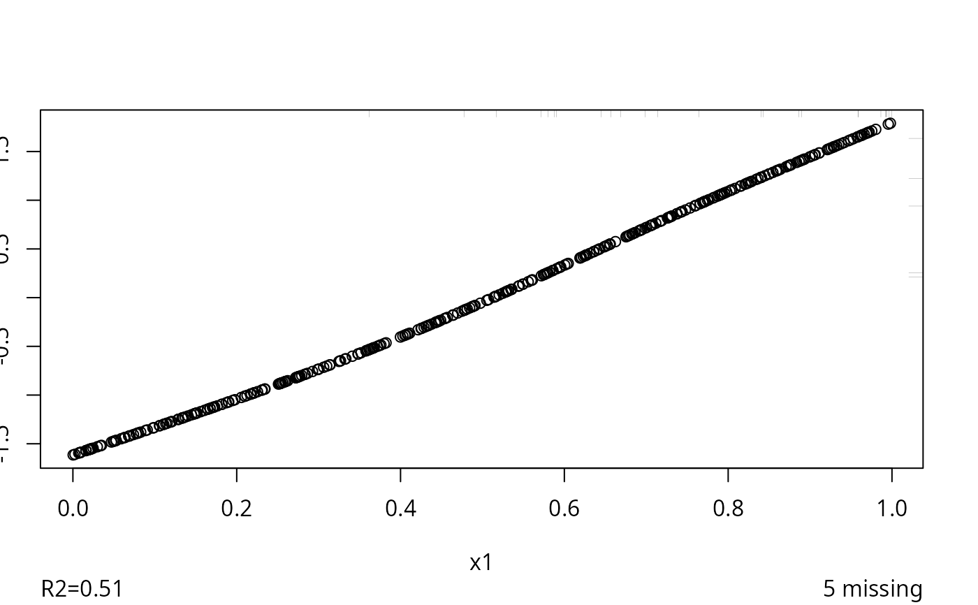
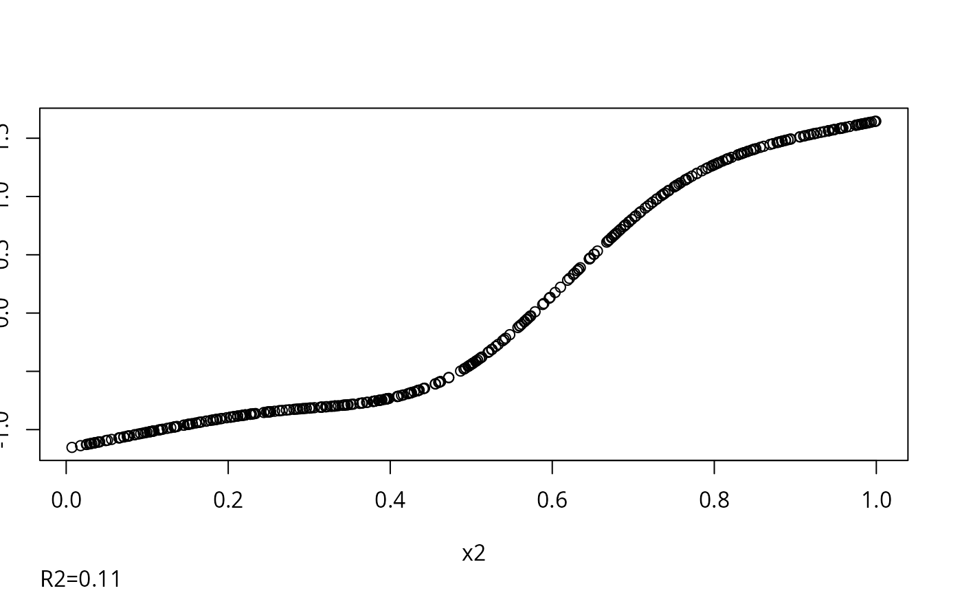
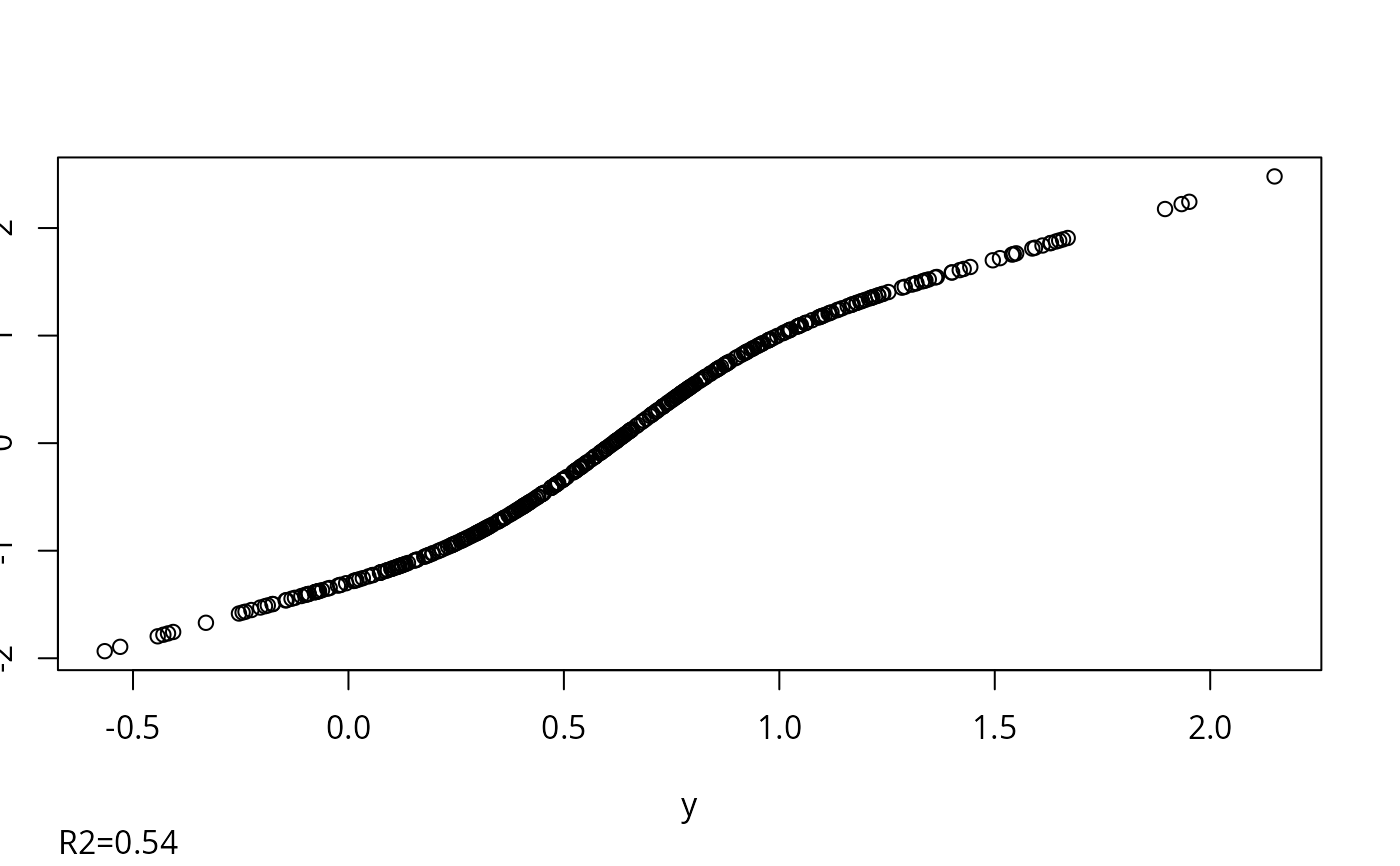
y <- x1*x2 + x1/(1+x2) + rnorm(n)/3
x1[1:5] <- NA
d <- data.frame(x1,x2,y)
w <- transcan(~ x1 + x2 + y, n.impute=5, data=d)
#> Warning: transcan provides only an approximation to true multiple imputation.
#> A better approximation is provided by the aregImpute function.
#> The MICE and other S libraries provide imputations from Bayesian posterior distributions.
#> Convergence criterion:0.167 0.025
#> 0.008
#> Convergence in 3 iterations
#> R-squared achieved in predicting each variable:
#>
#> x1 x2
#> 0.618 0.658
#>
#> Adjusted R-squared:
#>
#> x1 x2
#> 0.608 0.650
imputed <- as.data.frame(impute(z, data=d, list.out=TRUE))
#>
#>
#> Imputed missing values with the following frequencies
#> and stored them in variables with their original names:
#>
#> x1 x2
#> 20 6
# Example where multiple imputations are for basic variables and
# modeling is done on variables derived from these
set.seed(137)
n <- 400
x1 <- runif(n)
x2 <- runif(n)
y <- x1*x2 + x1/(1+x2) + rnorm(n)/3
x1[1:5] <- NA
d <- data.frame(x1,x2,y)
w <- transcan(~ x1 + x2 + y, n.impute=5, data=d)
#> Warning: transcan provides only an approximation to true multiple imputation.
#> A better approximation is provided by the aregImpute function.
#> The MICE and other S libraries provide imputations from Bayesian posterior distributions.
#> Convergence criterion:0.167 0.025
 #> 0.002
#> Convergence in 4 iterations
#> R-squared achieved in predicting each variable:
#>
#> x1 x2 y
#> 0.507 0.114 0.542
#>
#> Adjusted R-squared:
#>
#> x1 x2 y
#> 0.497 0.096 0.533
# Add ,show.imputed.actual for graphical diagnostics
if (FALSE) { # \dontrun{
g <- fit.mult.impute(y ~ product + ratio, ols, w,
data=data.frame(x1,x2,y),
derived=expression({
product <- x1*x2
ratio <- x1/(1+x2)
print(cbind(x1,x2,x1*x2,product)[1:6,])}))
} # }
# Here's a method for creating a permanent data frame containing
# one set of imputed values for each variable specified to transcan
# that had at least one NA, and also containing all the variables
# in an original data frame. The following is based on the fact
# that the default output location for impute.transcan is
# given by the global environment
if (FALSE) { # \dontrun{
xt <- transcan(~. , data=mine,
imputed=TRUE, shrink=TRUE, n.impute=10, trantab=TRUE)
attach(mine, use.names=FALSE)
impute(xt, imputation=1) # use first imputation
# omit imputation= if using single imputation
detach(1, 'mine2')
} # }
# Example of using invertTabulated outside transcan
x <- c(1,2,3,4,5,6,7,8,9,10)
y <- c(1,2,3,4,5,5,5,5,9,10)
freq <- c(1,1,1,1,1,2,3,4,1,1)
# x=5,6,7,8 with prob. .1 .2 .3 .4 when y=5
# Within a tolerance of .05*(10-1) all y's match exactly
# so the distance measure does not play a role
set.seed(1) # so can reproduce
for(inverse in c('linearInterp','sample'))
print(table(invertTabulated(x, y, freq, rep(5,1000), inverse=inverse)))
#>
#> 6.5
#> 1000
#>
#> 5 6 7 8
#> 110 194 291 405
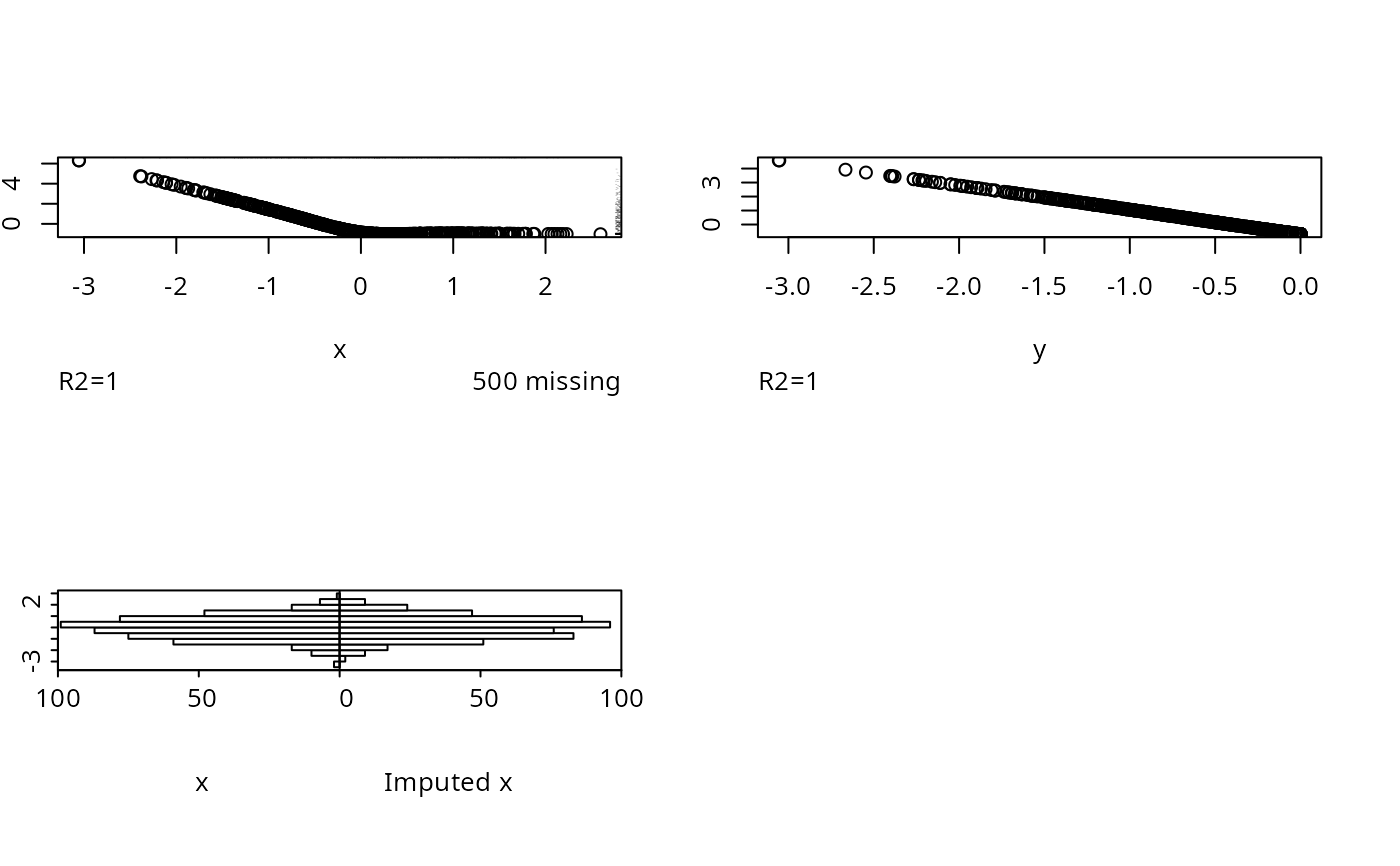
# Test inverse='sample' when the estimated transformation is
# flat on the right. First show default imputations
set.seed(3)
x <- rnorm(1000)
y <- pmin(x, 0)
x[1:500] <- NA
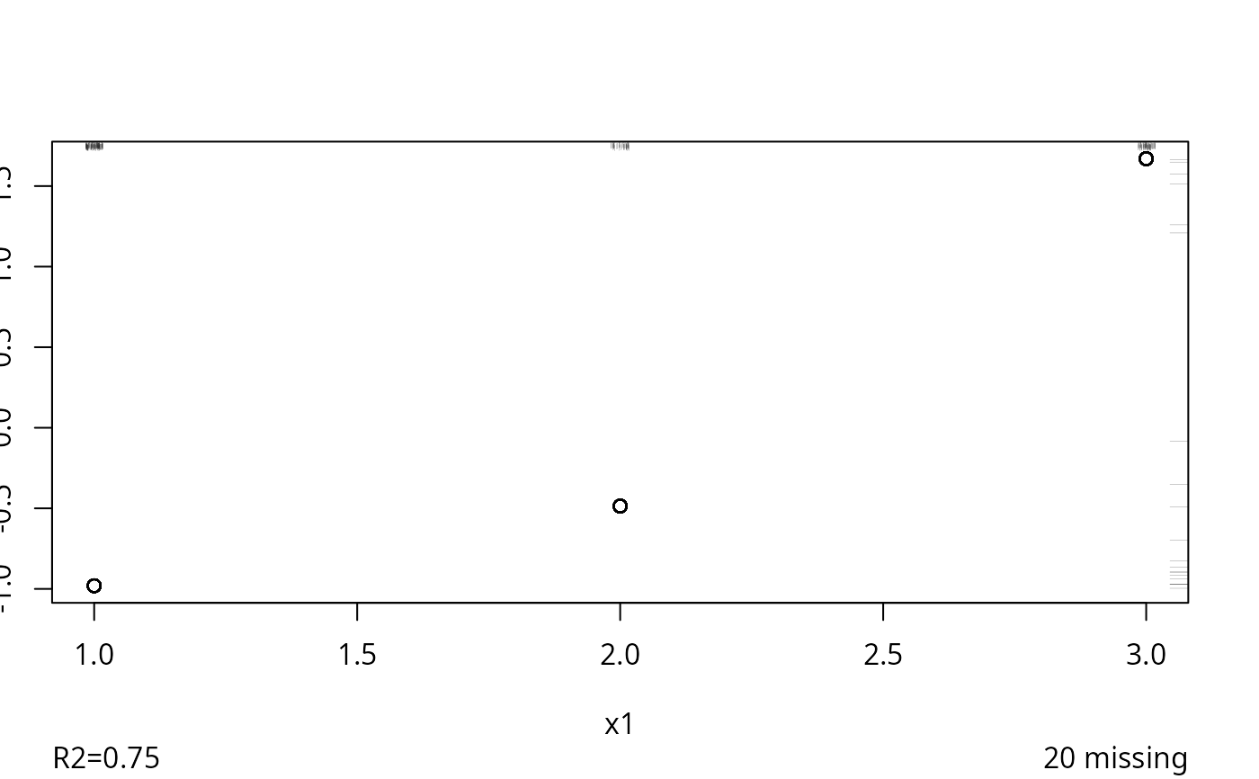
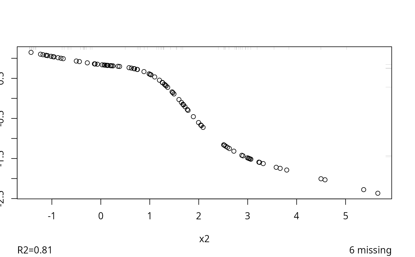
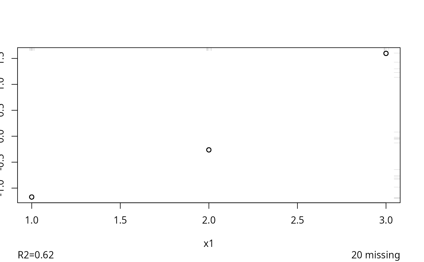
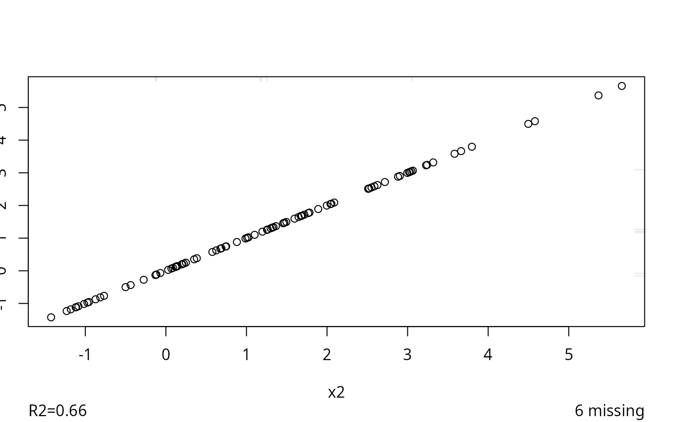
for(inverse in c('linearInterp','sample')) {
par(mfrow=c(2,2))
w <- transcan(~ x + y, imputed.actual='hist',
inverse=inverse, curtail=FALSE,
data=data.frame(x,y))
if(inverse=='sample') next
# cat('Click mouse on graph to proceed\n')
# locator(1)
}
#> Convergence criterion:0.032
#> 0.016
#> Convergence in 3 iterations
#> 0.002
#> Convergence in 4 iterations
#> R-squared achieved in predicting each variable:
#>
#> x1 x2 y
#> 0.507 0.114 0.542
#>
#> Adjusted R-squared:
#>
#> x1 x2 y
#> 0.497 0.096 0.533
# Add ,show.imputed.actual for graphical diagnostics
if (FALSE) { # \dontrun{
g <- fit.mult.impute(y ~ product + ratio, ols, w,
data=data.frame(x1,x2,y),
derived=expression({
product <- x1*x2
ratio <- x1/(1+x2)
print(cbind(x1,x2,x1*x2,product)[1:6,])}))
} # }
# Here's a method for creating a permanent data frame containing
# one set of imputed values for each variable specified to transcan
# that had at least one NA, and also containing all the variables
# in an original data frame. The following is based on the fact
# that the default output location for impute.transcan is
# given by the global environment
if (FALSE) { # \dontrun{
xt <- transcan(~. , data=mine,
imputed=TRUE, shrink=TRUE, n.impute=10, trantab=TRUE)
attach(mine, use.names=FALSE)
impute(xt, imputation=1) # use first imputation
# omit imputation= if using single imputation
detach(1, 'mine2')
} # }
# Example of using invertTabulated outside transcan
x <- c(1,2,3,4,5,6,7,8,9,10)
y <- c(1,2,3,4,5,5,5,5,9,10)
freq <- c(1,1,1,1,1,2,3,4,1,1)
# x=5,6,7,8 with prob. .1 .2 .3 .4 when y=5
# Within a tolerance of .05*(10-1) all y's match exactly
# so the distance measure does not play a role
set.seed(1) # so can reproduce
for(inverse in c('linearInterp','sample'))
print(table(invertTabulated(x, y, freq, rep(5,1000), inverse=inverse)))
#>
#> 6.5
#> 1000
#>
#> 5 6 7 8
#> 110 194 291 405
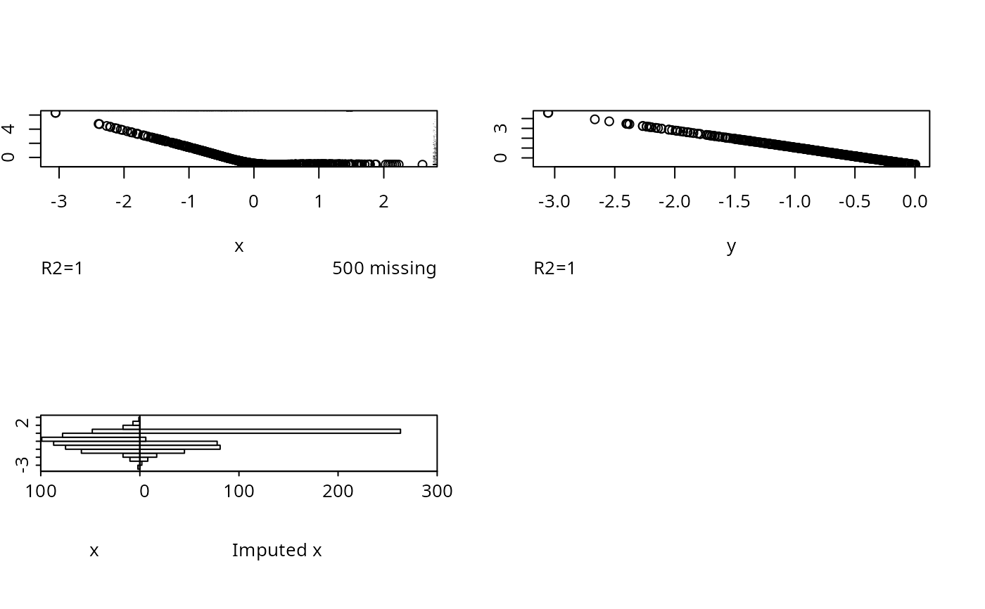
# Test inverse='sample' when the estimated transformation is
# flat on the right. First show default imputations
set.seed(3)
x <- rnorm(1000)
y <- pmin(x, 0)
x[1:500] <- NA
for(inverse in c('linearInterp','sample')) {
par(mfrow=c(2,2))
w <- transcan(~ x + y, imputed.actual='hist',
inverse=inverse, curtail=FALSE,
data=data.frame(x,y))
if(inverse=='sample') next
# cat('Click mouse on graph to proceed\n')
# locator(1)
}
#> Convergence criterion:0.032
#> 0.016
#> Convergence in 3 iterations
 #> R-squared achieved in predicting each variable:
#>
#> x y
#> 1 1
#>
#> Adjusted R-squared:
#>
#> x y
#> 1 1
#> Convergence criterion:0.032
#> Warning: No actual x has y value within 0.05* range(y) (7.35) of the following y values:5.4.
#> Consider increasing tolInverse. Used linear interpolation instead.
#> 0.016
#> Convergence in 3 iterations
#> R-squared achieved in predicting each variable:
#>
#> x y
#> 1 1
#>
#> Adjusted R-squared:
#>
#> x y
#> 1 1
if (FALSE) { # \dontrun{
# While running multiple imputation for a logistic regression model
# Run the rms package validate and calibrate functions and save the
# results in w$funresults
a <- aregImpute(~ x1 + x2 + y, data=d, n.impute=10)
require(rms)
g <- function(fit)
list(validate=validate(fit, B=50), calibrate=calibrate(fit, B=75))
w <- fit.mult.impute(y ~ x1 + x2, lrm, a, data=d, fun=g,
fitargs=list(x=TRUE, y=TRUE))
# Get all validate results in it's own list of length 10
r <- w$funresults
val <- lapply(r, function(x) x$validate)
cal <- lapply(r, function(x) x$calibrate)
# See rms processMI and https://hbiostat.org/rmsc/validate.html#sec-val-mival
} # }
if (FALSE) { # \dontrun{
# Account for within-subject correlation using the robust cluster sandwich
# covariance estimate in conjunction with Rubin's rule for multiple imputation
# rms package must be installed
a <- aregImpute(..., data=d)
f <- fit.mult.impute(y ~ x1 + x2, lrm, a, n.impute=30, data=d, cluster=d$id)
# Get likelihood ratio chi-square tests accounting for missingness
a <- aregImpute(..., data=d)
h <- fit.mult.impute(y ~ x1 + x2, lrm, a, n.impute=40, data=d, lrt=TRUE)
processMI(h, which='anova') # processMI is in rms
} # }
#> R-squared achieved in predicting each variable:
#>
#> x y
#> 1 1
#>
#> Adjusted R-squared:
#>
#> x y
#> 1 1
#> Convergence criterion:0.032
#> Warning: No actual x has y value within 0.05* range(y) (7.35) of the following y values:5.4.
#> Consider increasing tolInverse. Used linear interpolation instead.
#> 0.016
#> Convergence in 3 iterations
#> R-squared achieved in predicting each variable:
#>
#> x y
#> 1 1
#>
#> Adjusted R-squared:
#>
#> x y
#> 1 1
if (FALSE) { # \dontrun{
# While running multiple imputation for a logistic regression model
# Run the rms package validate and calibrate functions and save the
# results in w$funresults
a <- aregImpute(~ x1 + x2 + y, data=d, n.impute=10)
require(rms)
g <- function(fit)
list(validate=validate(fit, B=50), calibrate=calibrate(fit, B=75))
w <- fit.mult.impute(y ~ x1 + x2, lrm, a, data=d, fun=g,
fitargs=list(x=TRUE, y=TRUE))
# Get all validate results in it's own list of length 10
r <- w$funresults
val <- lapply(r, function(x) x$validate)
cal <- lapply(r, function(x) x$calibrate)
# See rms processMI and https://hbiostat.org/rmsc/validate.html#sec-val-mival
} # }
if (FALSE) { # \dontrun{
# Account for within-subject correlation using the robust cluster sandwich
# covariance estimate in conjunction with Rubin's rule for multiple imputation
# rms package must be installed
a <- aregImpute(..., data=d)
f <- fit.mult.impute(y ~ x1 + x2, lrm, a, n.impute=30, data=d, cluster=d$id)
# Get likelihood ratio chi-square tests accounting for missingness
a <- aregImpute(..., data=d)
h <- fit.mult.impute(y ~ x1 + x2, lrm, a, n.impute=40, data=d, lrt=TRUE)
processMI(h, which='anova') # processMI is in rms
} # }