Variable Clustering
varclus.RdDoes a hierarchical cluster analysis on variables, using the Hoeffding
D statistic, squared Pearson or Spearman correlations, or proportion
of observations for which two variables are both positive as similarity
measures. Variable clustering is used for assessing collinearity,
redundancy, and for separating variables into clusters that can be
scored as a single variable, thus resulting in data reduction. For
computing any of the three similarity measures, pairwise deletion of
NAs is done. The clustering is done by hclust(). A small function
naclus is also provided which depicts similarities in which
observations are missing for variables in a data frame. The
similarity measure is the fraction of NAs in common between any two
variables. The diagonals of this sim matrix are the fraction of NAs
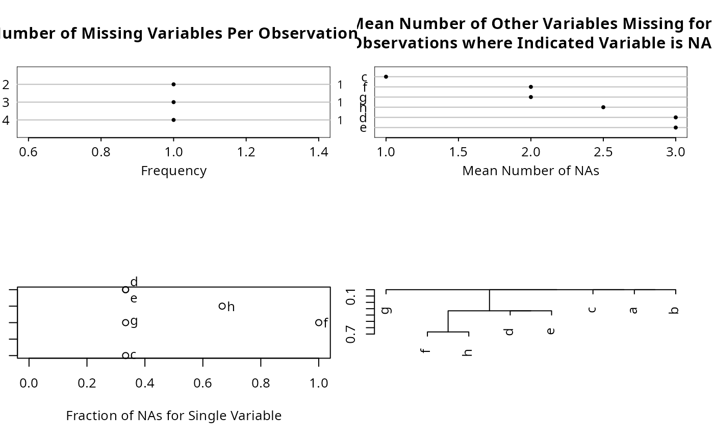
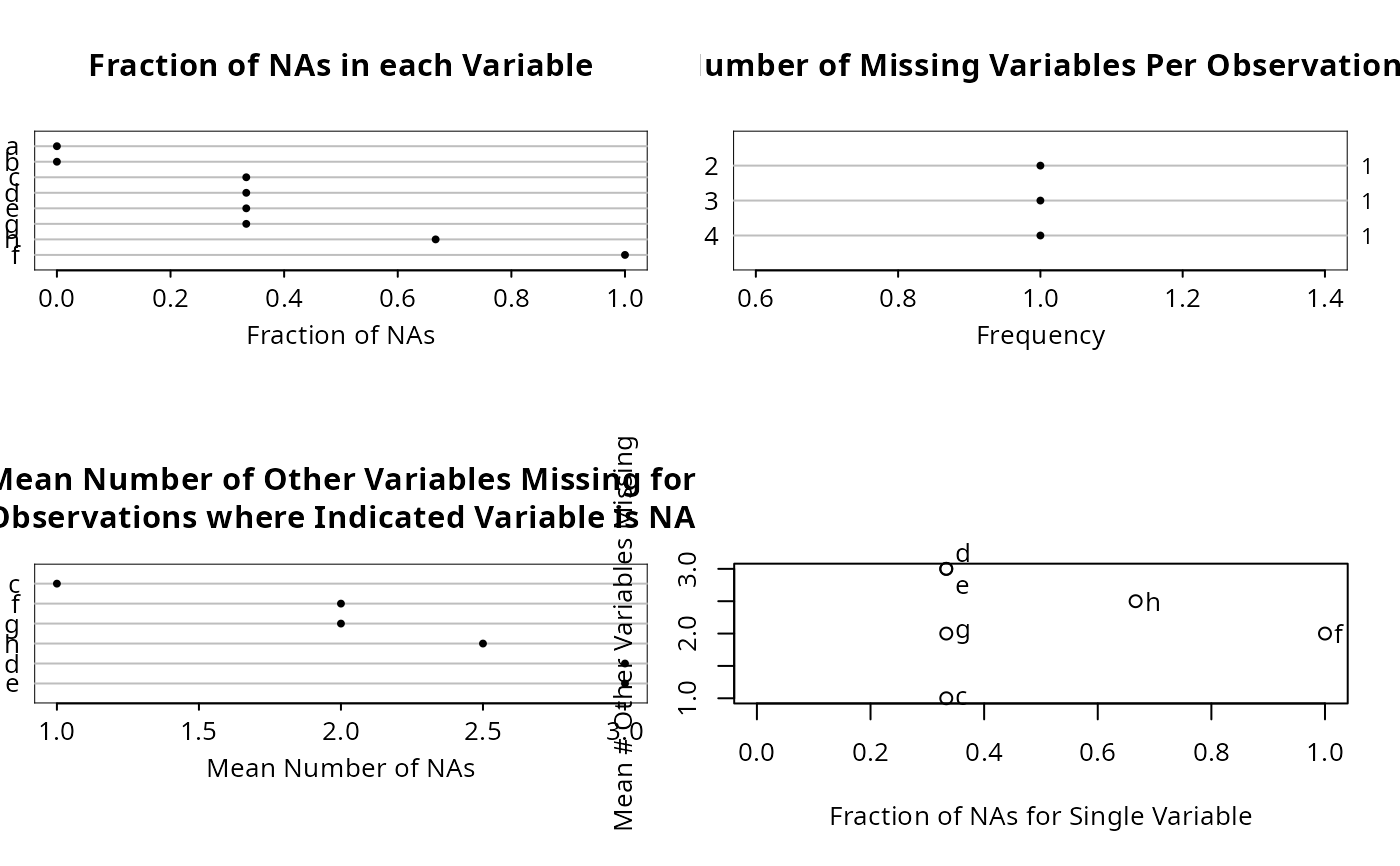
in each variable by itself. naclus also computes na.per.obs, the
number of missing variables in each observation, and mean.na, a
vector whose ith element is the mean number of missing variables other
than variable i, for observations in which variable i is missing. The
naplot function makes several plots (see the which argument).
So as to not generate too many dummy variables for multi-valued
character or categorical predictors, varclus will automatically
combine infrequent cells of such variables using
combine.levels.
plotMultSim plots multiple similarity matrices, with the similarity
measure being on the x-axis of each subplot.
na.pattern prints a frequency table of all combinations of
missingness for multiple variables. If there are 3 variables, a
frequency table entry labeled 110 corresponds to the number of
observations for which the first and second variables were missing but
the third variable was not missing.
Usage
varclus(x, similarity=c("spearman","pearson","hoeffding","bothpos","ccbothpos"),
        type=c("data.matrix","similarity.matrix"),
        method="complete",
        data=NULL, subset=NULL, na.action=na.retain,
        trans=c("square", "abs", "none"), ...)
# S3 method for class 'varclus'
print(x, abbrev=FALSE, ...)
# S3 method for class 'varclus'
plot(x, ylab, abbrev=FALSE, legend.=FALSE, loc, maxlen, labels, ...)

naclus(df, method)
naplot(obj, which=c('all','na per var','na per obs','mean na',
                    'na per var vs mean na'), ...)

plotMultSim(s, x=1:dim(s)[3],
            slim=range(pretty(c(0,max(s,na.rm=TRUE)))),
            slimds=FALSE,
            add=FALSE, lty=par('lty'), col=par('col'),
            lwd=par('lwd'), vname=NULL, h=.5, w=.75, u=.05,
            labelx=TRUE, xspace=.35)

na.pattern(x)
Arguments
- x
a formula, a numeric matrix of predictors, or a similarity matrix. If
xis a formula,model.matrixis used to convert it to a design matrix. If the formula excludes an intercept (e.g.,~ a + b -1), the first categorical (factor) variable in the formula will have dummy variables generated for all levels instead of omitting one for the first level. Forplotandprint,xis an object created byvarclus. Forna.pattern,xis a data table, data frame, or matrix.For
plotMultSim, is a numeric vector specifying the ordered unique values on the x-axis, corresponding to the third dimension ofs.- df
a data frame
- s
an array of similarity matrices. The third dimension of this array corresponds to different computations of similarities. The first two dimensions come from a single similarity matrix. This is useful for displaying similarity matrices computed by
varclus, for example. A use for this might be to show pairwise similarities of variables across time in a longitudinal study (see the example below). Ifvnameis not given,smust havedimnames.- similarity
the default is to use squared Spearman correlation coefficients, which will detect monotonic but nonlinear relationships. You can also specify linear correlation or Hoeffding's (1948) D statistic, which has the advantage of being sensitive to many types of dependence, including highly non-monotonic relationships. For binary data, or data to be made binary,
similarity="bothpos"uses as a similarity measure the proportion of observations for which two variables are both positive.similarity="ccbothpos"uses a chance-corrected measure which is the proportion of observations for which both variables are positive minus the product of the two marginal proportions. This difference is expected to be zero under independence. For diagonals,"ccbothpos"still uses the proportion of positives for the single variable. So"ccbothpos"is not really a similarity measure, and clustering is not done. This measure is useful for plotting withplotMultSim(see the last example).- type
if
xis not a formula, it may be a data matrix or a similarity matrix. By default, it is assumed to be a data matrix.- method
see
hclust. The default, for bothvarclusandnaclus, is"compact"(for R it is"complete").- data
a data frame, data table, or list
- subset
a standard subsetting expression
- na.action
These may be specified if
xis a formula. The defaultna.actionisna.retain, defined byvarclus. This causes all observations to be kept in the model frame, with later pairwise deletion ofNAs.- trans
By default, when the similarity measure is based on Pearson's or Spearman's correlation coefficients, the coefficients are squared. Specify
trans="abs"to take absolute values ortrans="none"to use the coefficients as they stand.- ...
for
varclusthese are optional arguments to pass to thedataframeReducefunction. Otherwise, passed toplclust(or todotchartordotchart2fornaplot).- ylab
y-axis label. Default is constructed on the basis of
similarity.- legend.
set to
TRUEto plot a legend defining the abbreviations- loc
a list with elements
xandydefining coordinates of the upper left corner of the legend. Default islocator(1).- maxlen
if a legend is plotted describing abbreviations, original labels longer than
maxlencharacters are truncated atmaxlen.- labels
a vector of character strings containing labels corresponding to columns in the similar matrix, if the column names of that matrix are not to be used
- obj
an object created by
naclus- which
defaults to
"all"meaning to havenaplotmake 4 separate plots. To make only one of the plots, usewhich="na per var"(dot chart of fraction of NAs for each variable), ,"na per obs"(dot chart showing frequency distribution of number of variables having NAs in an observation),"mean na"(dot chart showing mean number of other variables missing when the indicated variable is missing), or"na per var vs mean na", a scatterplot showing on the x-axis the fraction of NAs in the variable and on the y-axis the mean number of other variables that are NA when the indicated variable is NA.- abbrev
set to
TRUEto abbreviate variable names for plotting or printing. Is set toTRUEautomatically iflegend=TRUE.- slim
2-vector specifying the range of similarity values for scaling the y-axes. By default this is the observed range over all of
s.- slimds
set to
slimdstoTRUEto scale diagonals and off-diagonals separately- add
set to
TRUEto add similarities to an existing plot (usually specifyingltyorcol)- lty, col, lwd
line type, color, or line thickness for
plotMultSim- vname
optional vector of variable names, in order, used in
s- h
relative height for subplot
- w
relative width for subplot
- u
relative extra height and width to leave unused inside the subplot. Also used as the space between y-axis tick mark labels and graph border.
- labelx
set to
FALSEto suppress drawing of labels in the x direction- xspace
amount of space, on a scale of 1:
nwherenis the number of variables, to set aside for y-axis labels
Value
for varclus or naclus, a list of class varclus with elements
call (containing the calling statement), sim (similarity matrix),
n (sample size used if x was not a correlation matrix already -
n is a matrix), hclust, the object created by hclust,
similarity, and method. naclus also returns the
two vectors listed under
description, and naplot returns an invisible vector that is the
frequency table of the number of missing variables per observation.
plotMultSim invisibly returns the limits of similarities used in
constructing the y-axes of each subplot. For similarity="ccbothpos"
the hclust object is NULL.
na.pattern creates an integer vector of frequencies.
Details
options(contrasts= c("contr.treatment", "contr.poly")) is issued
temporarily by varclus to make sure that ordinary dummy variables
are generated for factor variables. Pass arguments to the
dataframeReduce function to remove problematic variables
(especially if analyzing all variables in a data frame).
Author
Frank Harrell
Department of Biostatistics, Vanderbilt University
fh@fharrell.com
References
Sarle, WS: The VARCLUS Procedure. SAS/STAT User's Guide, 4th Edition, 1990. Cary NC: SAS Institute, Inc.
Hoeffding W. (1948): A non-parametric test of independence. Ann Math Stat 19:546–57.
See also
hclust, plclust, hoeffd, rcorr, cor, model.matrix,
locator, na.pattern, cut2, combine.levels
Examples
set.seed(1)
x1 <- rnorm(200)
x2 <- rnorm(200)
x3 <- x1 + x2 + rnorm(200)
x4 <- x2 + rnorm(200)
x <- cbind(x1,x2,x3,x4)
v <- varclus(x, similarity="spear") # spearman is the default anyway
v # invokes print.varclus
#> varclus(x = x, similarity = "spear")
#>
#>
#> Similarity matrix (Spearman rho^2)
#>
#> x1 x2 x3 x4
#> x1 1.00 0.00 0.26 0.00
#> x2 0.00 1.00 0.26 0.42
#> x3 0.26 0.26 1.00 0.12
#> x4 0.00 0.42 0.12 1.00
#>
#> No. of observations used for each pair:
#>
#> x1 x2 x3 x4
#> x1 200 200 200 200
#> x2 200 200 200 200
#> x3 200 200 200 200
#> x4 200 200 200 200
#>
#> hclust results (method=complete)
#>
#>
#> Call:
#> hclust(d = as.dist(1 - x), method = method)
#>
#> Cluster method : complete
#> Number of objects: 4
#>
print(round(v$sim,2))
#> x1 x2 x3 x4
#> x1 1.00 0.00 0.26 0.00
#> x2 0.00 1.00 0.26 0.42
#> x3 0.26 0.26 1.00 0.12
#> x4 0.00 0.42 0.12 1.00
plot(v)
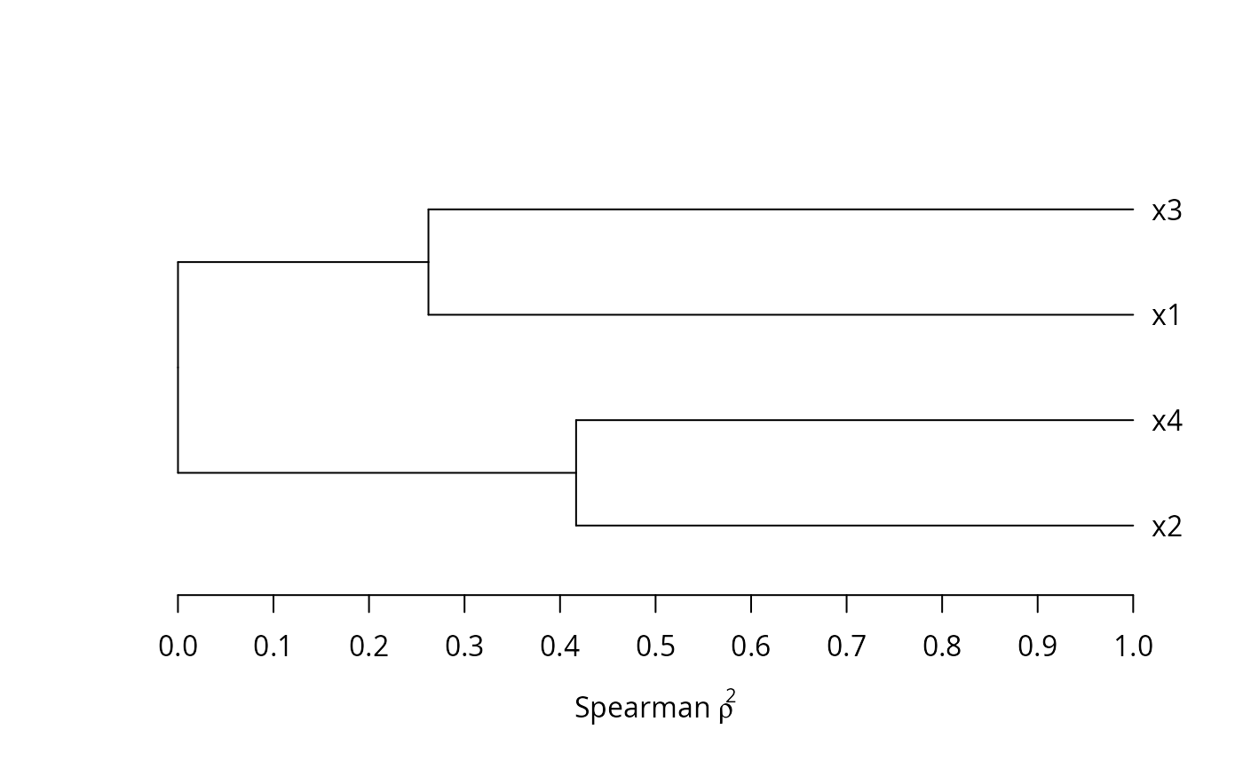
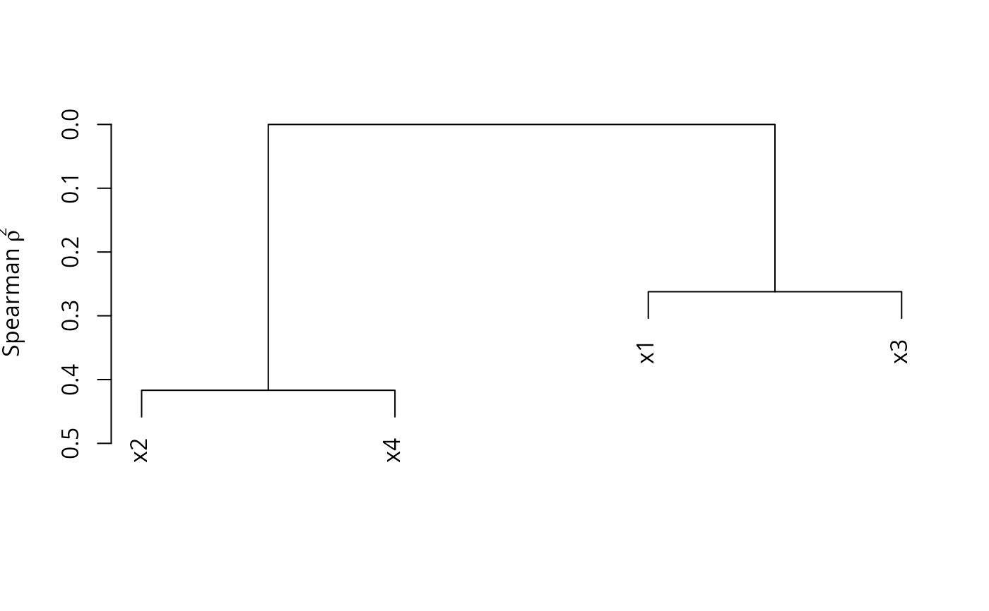 # Convert the dendrogram to be horizontal
v <- as.dendrogram(v$hclust)
plot(v, horiz=TRUE, axes=FALSE, xlab=expression(paste('Spearman ', rho^2)))
rh <- seq(0, 1, by=0.1) # re-label x-axis re:similarity not distance
axis(1, at=1 - rh, labels=format(rh))
# Convert the dendrogram to be horizontal
v <- as.dendrogram(v$hclust)
plot(v, horiz=TRUE, axes=FALSE, xlab=expression(paste('Spearman ', rho^2)))
rh <- seq(0, 1, by=0.1) # re-label x-axis re:similarity not distance
axis(1, at=1 - rh, labels=format(rh))
 # plot(varclus(~ age + sys.bp + dias.bp + country - 1), abbrev=TRUE)
# the -1 causes k dummies to be generated for k countries
# plot(varclus(~ age + factor(disease.code) - 1))
#
#
# use varclus(~., data= fracmiss= maxlevels= minprev=) to analyze all
# "useful" variables - see dataframeReduce for details about arguments
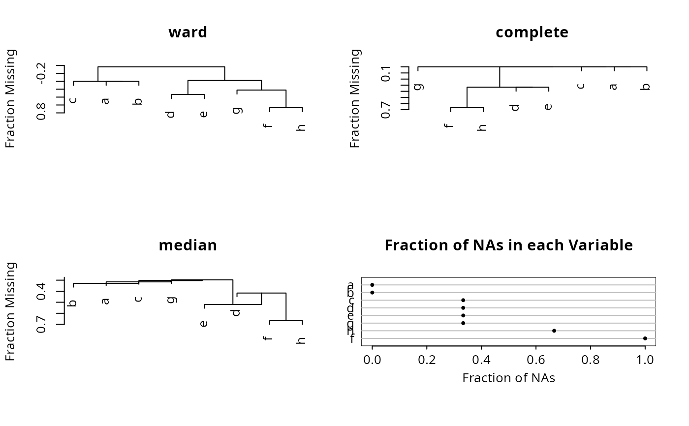
df <- data.frame(a=c(1,2,3),b=c(1,2,3),c=c(1,2,NA),d=c(1,NA,3),
e=c(1,NA,3),f=c(NA,NA,NA),g=c(NA,2,3),h=c(NA,NA,3))
par(mfrow=c(2,2))
for(m in c("ward","complete","median")) {
plot(naclus(df, method=m))
title(m)
}
#> The "ward" method has been renamed to "ward.D"; note new "ward.D2"
naplot(naclus(df))
# plot(varclus(~ age + sys.bp + dias.bp + country - 1), abbrev=TRUE)
# the -1 causes k dummies to be generated for k countries
# plot(varclus(~ age + factor(disease.code) - 1))
#
#
# use varclus(~., data= fracmiss= maxlevels= minprev=) to analyze all
# "useful" variables - see dataframeReduce for details about arguments
df <- data.frame(a=c(1,2,3),b=c(1,2,3),c=c(1,2,NA),d=c(1,NA,3),
e=c(1,NA,3),f=c(NA,NA,NA),g=c(NA,2,3),h=c(NA,NA,3))
par(mfrow=c(2,2))
for(m in c("ward","complete","median")) {
plot(naclus(df, method=m))
title(m)
}
#> The "ward" method has been renamed to "ward.D"; note new "ward.D2"
naplot(naclus(df))
 n <- naclus(df)
plot(n); naplot(n)
n <- naclus(df)
plot(n); naplot(n)
 na.pattern(df)
#> pattern
#> 00000111 00011101 00100100
#> 1 1 1
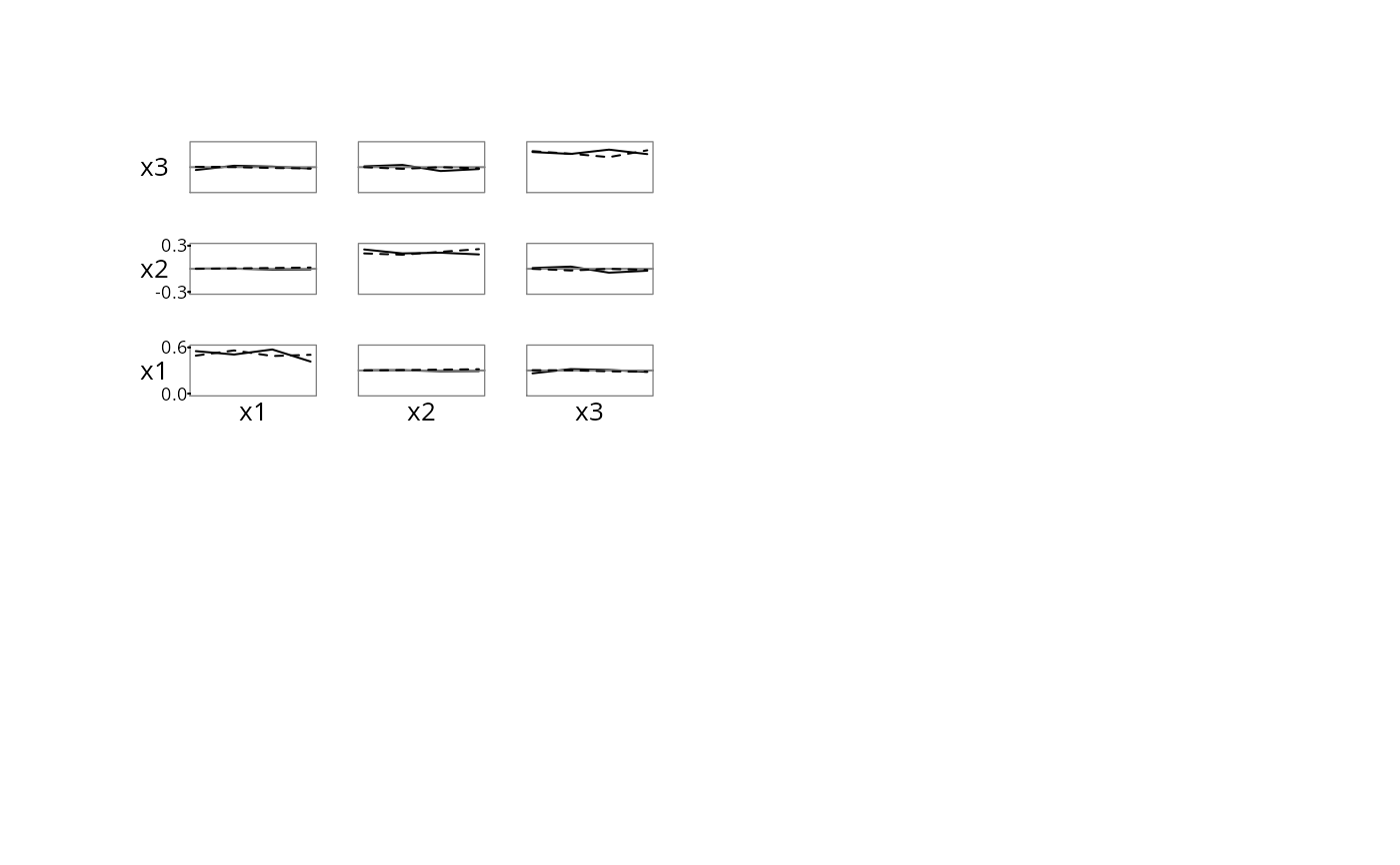
# plotMultSim example: Plot proportion of observations
# for which two variables are both positive (diagonals
# show the proportion of observations for which the
# one variable is positive). Chance-correct the
# off-diagonals by subtracting the product of the
# marginal proportions. On each subplot the x-axis
# shows month (0, 4, 8, 12) and there is a separate
# curve for females and males
d <- data.frame(sex=sample(c('female','male'),1000,TRUE),
month=sample(c(0,4,8,12),1000,TRUE),
x1=sample(0:1,1000,TRUE),
x2=sample(0:1,1000,TRUE),
x3=sample(0:1,1000,TRUE))
s <- array(NA, c(3,3,4))
opar <- par(mar=c(0,0,4.1,0)) # waste less space
for(sx in c('female','male')) {
for(i in 1:4) {
mon <- (i-1)*4
s[,,i] <- varclus(~x1 + x2 + x3, sim='ccbothpos', data=d,
subset=d$month==mon & d$sex==sx)$sim
}
plotMultSim(s, c(0,4,8,12), vname=c('x1','x2','x3'),
add=sx=='male', slimds=TRUE,
lty=1+(sx=='male'))
# slimds=TRUE causes separate scaling for diagonals and
# off-diagonals
}
par(opar)
na.pattern(df)
#> pattern
#> 00000111 00011101 00100100
#> 1 1 1
# plotMultSim example: Plot proportion of observations
# for which two variables are both positive (diagonals
# show the proportion of observations for which the
# one variable is positive). Chance-correct the
# off-diagonals by subtracting the product of the
# marginal proportions. On each subplot the x-axis
# shows month (0, 4, 8, 12) and there is a separate
# curve for females and males
d <- data.frame(sex=sample(c('female','male'),1000,TRUE),
month=sample(c(0,4,8,12),1000,TRUE),
x1=sample(0:1,1000,TRUE),
x2=sample(0:1,1000,TRUE),
x3=sample(0:1,1000,TRUE))
s <- array(NA, c(3,3,4))
opar <- par(mar=c(0,0,4.1,0)) # waste less space
for(sx in c('female','male')) {
for(i in 1:4) {
mon <- (i-1)*4
s[,,i] <- varclus(~x1 + x2 + x3, sim='ccbothpos', data=d,
subset=d$month==mon & d$sex==sx)$sim
}
plotMultSim(s, c(0,4,8,12), vname=c('x1','x2','x3'),
add=sx=='male', slimds=TRUE,
lty=1+(sx=='male'))
# slimds=TRUE causes separate scaling for diagonals and
# off-diagonals
}
par(opar)