Data and Examples from Franses (1998)
Franses1998.RdThis manual page collects a list of examples from the book. Some solutions might not be exact and the list is certainly not complete. If you have suggestions for improvement (preferably in the form of code), please contact the package maintainer.
References
Franses, P.H. (1998). Time Series Models for Business and Economic Forecasting. Cambridge, UK: Cambridge University Press.
Examples
###########################
## Convenience functions ##
###########################
## EACF tables (Franses 1998, p. 99)
ctrafo <- function(x) residuals(lm(x ~ factor(cycle(x))))
ddiff <- function(x) diff(diff(x, frequency(x)), 1)
eacf <- function(y, lag = 12) {
stopifnot(all(lag > 0))
if(length(lag) < 2) lag <- 1:lag
rval <- sapply(
list(y = y, dy = diff(y), cdy = ctrafo(diff(y)),
Dy = diff(y, frequency(y)), dDy = ddiff(y)),
function(x) acf(x, plot = FALSE, lag.max = max(lag))$acf[lag + 1])
rownames(rval) <- lag
return(rval)
}
#######################################
## Index of US industrial production ##
#######################################
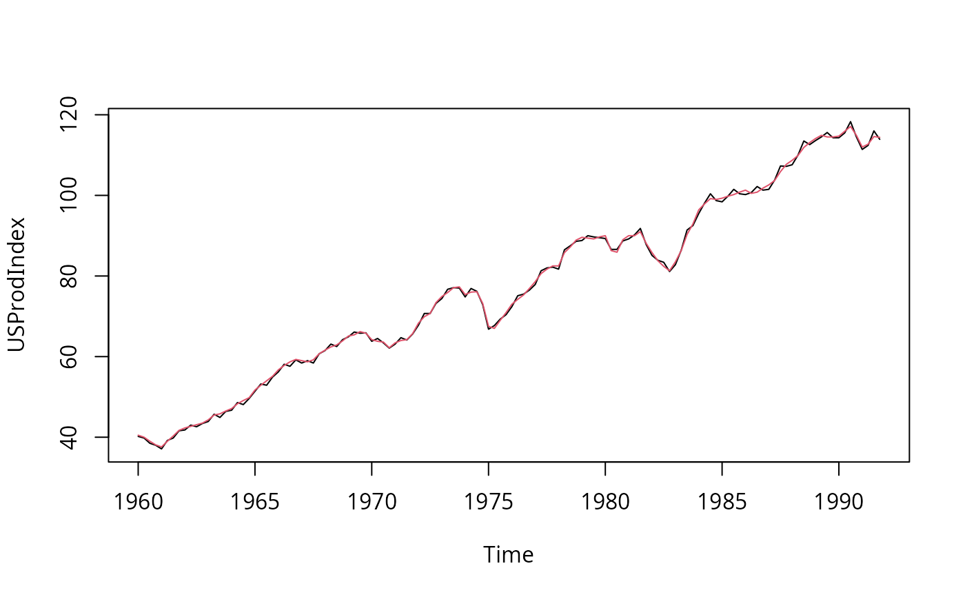
data("USProdIndex", package = "AER")
plot(USProdIndex, plot.type = "single", col = 1:2)
 ## Franses (1998), Table 5.1
round(eacf(log(USProdIndex[,1])), digits = 3)
#> y dy cdy Dy dDy
#> 1 0.975 0.162 0.242 0.851 0.535
#> 2 0.947 0.140 0.196 0.586 0.162
#> 3 0.918 -0.110 -0.061 0.295 -0.051
#> 4 0.888 0.300 0.205 0.036 -0.328
#> 5 0.853 -0.268 -0.264 -0.126 -0.296
#> 6 0.821 -0.046 -0.032 -0.220 -0.190
#> 7 0.789 -0.249 -0.224 -0.274 -0.165
#> 8 0.761 0.120 0.008 -0.296 -0.204
#> 9 0.732 -0.257 -0.253 -0.262 -0.066
#> 10 0.705 0.015 0.044 -0.207 0.080
#> 11 0.676 -0.198 -0.165 -0.172 0.025
#> 12 0.649 0.199 0.099 -0.138 0.018
## Franses (1998), Equation 5.6: Unrestricted airline model
## (Franses: ma1 = 0.388 (0.063), ma4 = -0.739 (0.060), ma5 = -0.452 (0.069))
arima(log(USProdIndex[,1]), c(0, 1, 5), c(0, 1, 0), fixed = c(NA, 0, 0, NA, NA))
#>
#> Call:
#> arima(x = log(USProdIndex[, 1]), order = c(0, 1, 5), seasonal = c(0, 1, 0),
#> fixed = c(NA, 0, 0, NA, NA))
#>
#> Coefficients:
#> ma1 ma2 ma3 ma4 ma5
#> 0.4603 0 0 -0.7731 -0.5313
#> s.e. 0.0707 0 0 0.0626 0.0713
#>
#> sigma^2 estimated as 0.0003366: log likelihood = 314.84, aic = -621.69
###########################################
## Consumption of non-durables in the UK ##
###########################################
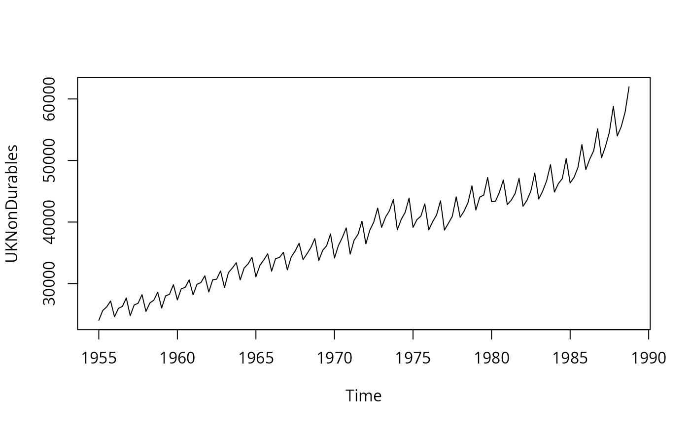
data("UKNonDurables", package = "AER")
plot(UKNonDurables)
## Franses (1998), Table 5.1
round(eacf(log(USProdIndex[,1])), digits = 3)
#> y dy cdy Dy dDy
#> 1 0.975 0.162 0.242 0.851 0.535
#> 2 0.947 0.140 0.196 0.586 0.162
#> 3 0.918 -0.110 -0.061 0.295 -0.051
#> 4 0.888 0.300 0.205 0.036 -0.328
#> 5 0.853 -0.268 -0.264 -0.126 -0.296
#> 6 0.821 -0.046 -0.032 -0.220 -0.190
#> 7 0.789 -0.249 -0.224 -0.274 -0.165
#> 8 0.761 0.120 0.008 -0.296 -0.204
#> 9 0.732 -0.257 -0.253 -0.262 -0.066
#> 10 0.705 0.015 0.044 -0.207 0.080
#> 11 0.676 -0.198 -0.165 -0.172 0.025
#> 12 0.649 0.199 0.099 -0.138 0.018
## Franses (1998), Equation 5.6: Unrestricted airline model
## (Franses: ma1 = 0.388 (0.063), ma4 = -0.739 (0.060), ma5 = -0.452 (0.069))
arima(log(USProdIndex[,1]), c(0, 1, 5), c(0, 1, 0), fixed = c(NA, 0, 0, NA, NA))
#>
#> Call:
#> arima(x = log(USProdIndex[, 1]), order = c(0, 1, 5), seasonal = c(0, 1, 0),
#> fixed = c(NA, 0, 0, NA, NA))
#>
#> Coefficients:
#> ma1 ma2 ma3 ma4 ma5
#> 0.4603 0 0 -0.7731 -0.5313
#> s.e. 0.0707 0 0 0.0626 0.0713
#>
#> sigma^2 estimated as 0.0003366: log likelihood = 314.84, aic = -621.69
###########################################
## Consumption of non-durables in the UK ##
###########################################
data("UKNonDurables", package = "AER")
plot(UKNonDurables)
 ## Franses (1998), Table 5.2
round(eacf(log(UKNonDurables)), digits = 3)
#> y dy cdy Dy dDy
#> 1 0.928 -0.463 -0.074 0.779 -0.164
#> 2 0.900 -0.014 -0.359 0.625 0.050
#> 3 0.876 -0.481 -0.034 0.449 0.048
#> 4 0.891 0.947 0.554 0.248 -0.444
#> 5 0.823 -0.438 0.023 0.238 0.236
#> 6 0.795 -0.014 -0.390 0.130 -0.118
#> 7 0.771 -0.471 -0.045 0.082 0.115
#> 8 0.788 0.910 0.491 -0.014 0.023
#> 9 0.723 -0.421 -0.081 -0.125 -0.251
#> 10 0.697 -0.014 -0.328 -0.133 0.122
#> 11 0.674 -0.464 -0.148 -0.196 -0.131
#> 12 0.691 0.877 0.414 -0.196 -0.001
## Franses (1998), Equation 5.51
## (Franses: sma1 = -0.632 (0.069))
arima(log(UKNonDurables), c(0, 1, 0), c(0, 1, 1))
#>
#> Call:
#> arima(x = log(UKNonDurables), order = c(0, 1, 0), seasonal = c(0, 1, 1))
#>
#> Coefficients:
#> sma1
#> -0.6095
#> s.e. 0.0711
#>
#> sigma^2 estimated as 0.0001234: log likelihood = 402.71, aic = -801.42
##############################
## Dutch retail sales index ##
##############################
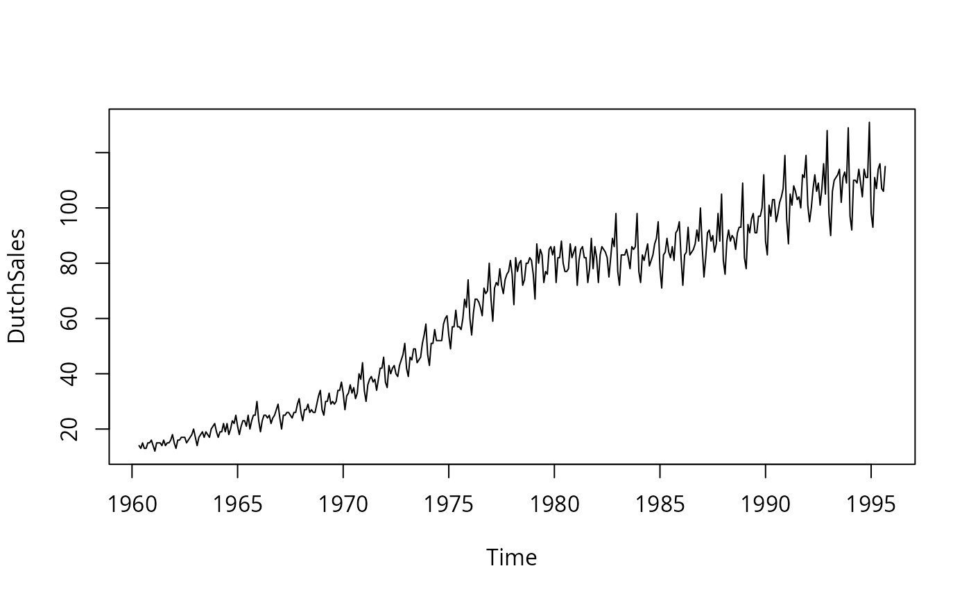
data("DutchSales", package = "AER")
plot(DutchSales)
## Franses (1998), Table 5.2
round(eacf(log(UKNonDurables)), digits = 3)
#> y dy cdy Dy dDy
#> 1 0.928 -0.463 -0.074 0.779 -0.164
#> 2 0.900 -0.014 -0.359 0.625 0.050
#> 3 0.876 -0.481 -0.034 0.449 0.048
#> 4 0.891 0.947 0.554 0.248 -0.444
#> 5 0.823 -0.438 0.023 0.238 0.236
#> 6 0.795 -0.014 -0.390 0.130 -0.118
#> 7 0.771 -0.471 -0.045 0.082 0.115
#> 8 0.788 0.910 0.491 -0.014 0.023
#> 9 0.723 -0.421 -0.081 -0.125 -0.251
#> 10 0.697 -0.014 -0.328 -0.133 0.122
#> 11 0.674 -0.464 -0.148 -0.196 -0.131
#> 12 0.691 0.877 0.414 -0.196 -0.001
## Franses (1998), Equation 5.51
## (Franses: sma1 = -0.632 (0.069))
arima(log(UKNonDurables), c(0, 1, 0), c(0, 1, 1))
#>
#> Call:
#> arima(x = log(UKNonDurables), order = c(0, 1, 0), seasonal = c(0, 1, 1))
#>
#> Coefficients:
#> sma1
#> -0.6095
#> s.e. 0.0711
#>
#> sigma^2 estimated as 0.0001234: log likelihood = 402.71, aic = -801.42
##############################
## Dutch retail sales index ##
##############################
data("DutchSales", package = "AER")
plot(DutchSales)
 ## Franses (1998), Table 5.3
round(eacf(log(DutchSales), lag = c(1:18, 24, 36)), digits = 3)
#> y dy cdy Dy dDy
#> 1 0.980 -0.264 -0.556 0.456 -0.532
#> 2 0.967 -0.238 -0.024 0.490 -0.121
#> 3 0.961 -0.004 0.221 0.654 0.307
#> 4 0.954 -0.256 -0.180 0.486 -0.200
#> 5 0.954 0.163 0.010 0.534 -0.011
#> 6 0.950 0.236 0.160 0.593 0.148
#> 7 0.940 0.093 -0.150 0.492 -0.093
#> 8 0.929 -0.195 -0.025 0.492 -0.106
#> 9 0.922 -0.004 0.223 0.607 0.268
#> 10 0.912 -0.306 -0.256 0.431 -0.276
#> 11 0.913 -0.098 -0.035 0.556 0.228
#> 12 0.916 0.816 0.453 0.432 -0.061
#> 13 0.897 -0.248 -0.497 0.375 -0.290
#> 14 0.885 -0.113 0.344 0.633 0.408
#> 15 0.877 -0.112 -0.125 0.446 -0.119
#> 16 0.870 -0.238 -0.109 0.392 -0.189
#> 17 0.870 0.218 0.176 0.540 0.240
#> 18 0.865 0.181 -0.008 0.429 -0.045
#> 24 0.827 0.656 -0.007 0.300 -0.308
#> 36 0.738 0.593 -0.125 0.210 -0.312
###########################################
## TV and radio advertising expenditures ##
###########################################
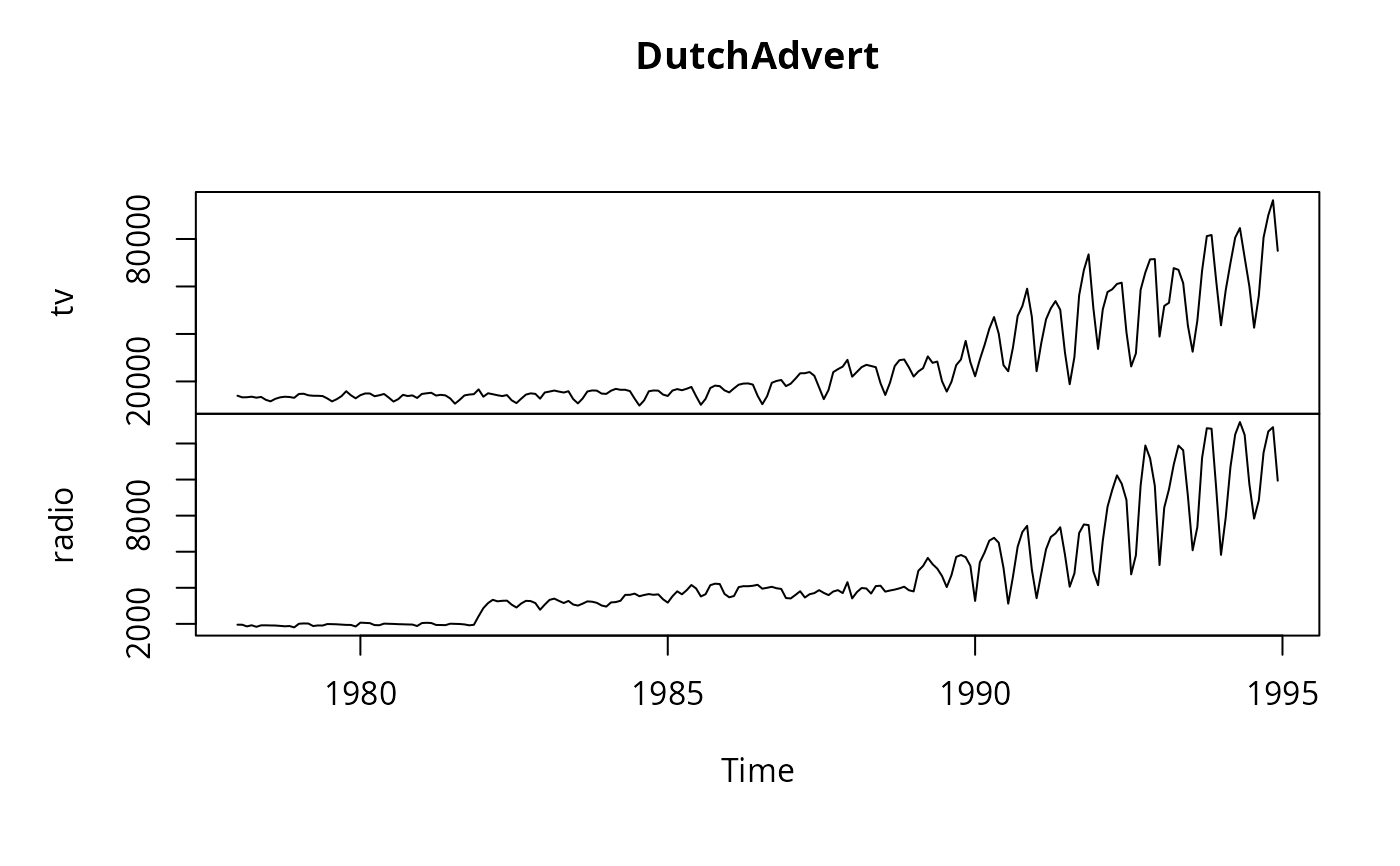
data("DutchAdvert", package = "AER")
plot(DutchAdvert)
## Franses (1998), Table 5.3
round(eacf(log(DutchSales), lag = c(1:18, 24, 36)), digits = 3)
#> y dy cdy Dy dDy
#> 1 0.980 -0.264 -0.556 0.456 -0.532
#> 2 0.967 -0.238 -0.024 0.490 -0.121
#> 3 0.961 -0.004 0.221 0.654 0.307
#> 4 0.954 -0.256 -0.180 0.486 -0.200
#> 5 0.954 0.163 0.010 0.534 -0.011
#> 6 0.950 0.236 0.160 0.593 0.148
#> 7 0.940 0.093 -0.150 0.492 -0.093
#> 8 0.929 -0.195 -0.025 0.492 -0.106
#> 9 0.922 -0.004 0.223 0.607 0.268
#> 10 0.912 -0.306 -0.256 0.431 -0.276
#> 11 0.913 -0.098 -0.035 0.556 0.228
#> 12 0.916 0.816 0.453 0.432 -0.061
#> 13 0.897 -0.248 -0.497 0.375 -0.290
#> 14 0.885 -0.113 0.344 0.633 0.408
#> 15 0.877 -0.112 -0.125 0.446 -0.119
#> 16 0.870 -0.238 -0.109 0.392 -0.189
#> 17 0.870 0.218 0.176 0.540 0.240
#> 18 0.865 0.181 -0.008 0.429 -0.045
#> 24 0.827 0.656 -0.007 0.300 -0.308
#> 36 0.738 0.593 -0.125 0.210 -0.312
###########################################
## TV and radio advertising expenditures ##
###########################################
data("DutchAdvert", package = "AER")
plot(DutchAdvert)
 ## Franses (1998), Table 5.4
round(eacf(log(DutchAdvert[,"tv"]), lag = c(1:19, 26, 39)), digits = 3)
#> y dy cdy Dy dDy
#> 1 0.933 0.215 0.039 0.663 -0.301
#> 2 0.836 -0.352 -0.255 0.529 -0.111
#> 3 0.781 -0.418 -0.316 0.471 -0.083
#> 4 0.774 -0.351 -0.301 0.466 0.044
#> 5 0.813 -0.013 -0.020 0.431 0.001
#> 6 0.857 0.417 0.346 0.393 -0.003
#> 7 0.848 0.438 0.409 0.357 0.036
#> 8 0.786 -0.008 0.024 0.299 0.008
#> 9 0.723 -0.348 -0.308 0.233 -0.031
#> 10 0.700 -0.398 -0.288 0.191 -0.022
#> 11 0.725 -0.324 -0.191 0.162 0.026
#> 12 0.788 0.240 0.109 0.119 0.105
#> 13 0.829 0.810 0.531 0.004 -0.412
#> 14 0.773 0.265 0.183 0.172 0.312
#> 15 0.683 -0.331 -0.210 0.125 -0.103
#> 16 0.630 -0.370 -0.222 0.146 0.096
#> 17 0.621 -0.334 -0.277 0.103 0.008
#> 18 0.656 -0.025 -0.053 0.050 -0.187
#> 19 0.699 0.383 0.274 0.127 0.003
#> 26 0.672 0.728 0.399 0.111 -0.002
#> 39 0.500 0.650 0.294 0.172 0.034
## Franses (1998), Table 5.4
round(eacf(log(DutchAdvert[,"tv"]), lag = c(1:19, 26, 39)), digits = 3)
#> y dy cdy Dy dDy
#> 1 0.933 0.215 0.039 0.663 -0.301
#> 2 0.836 -0.352 -0.255 0.529 -0.111
#> 3 0.781 -0.418 -0.316 0.471 -0.083
#> 4 0.774 -0.351 -0.301 0.466 0.044
#> 5 0.813 -0.013 -0.020 0.431 0.001
#> 6 0.857 0.417 0.346 0.393 -0.003
#> 7 0.848 0.438 0.409 0.357 0.036
#> 8 0.786 -0.008 0.024 0.299 0.008
#> 9 0.723 -0.348 -0.308 0.233 -0.031
#> 10 0.700 -0.398 -0.288 0.191 -0.022
#> 11 0.725 -0.324 -0.191 0.162 0.026
#> 12 0.788 0.240 0.109 0.119 0.105
#> 13 0.829 0.810 0.531 0.004 -0.412
#> 14 0.773 0.265 0.183 0.172 0.312
#> 15 0.683 -0.331 -0.210 0.125 -0.103
#> 16 0.630 -0.370 -0.222 0.146 0.096
#> 17 0.621 -0.334 -0.277 0.103 0.008
#> 18 0.656 -0.025 -0.053 0.050 -0.187
#> 19 0.699 0.383 0.274 0.127 0.003
#> 26 0.672 0.728 0.399 0.111 -0.002
#> 39 0.500 0.650 0.294 0.172 0.034