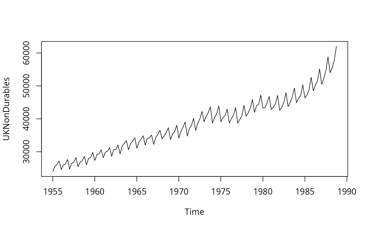
Consumption of Non-Durables in the UK

Time series of consumption of non-durables in the UK (in 1985 prices).

Usage

data("UKNonDurables")

Format

A quarterly univariate time series from 1955(1) to 1988(4).

Source

Online complements to Franses (1998).

References

Osborn, D.R. (1988). A Survey of Seasonality in UK Macroeconomic Variables. International Journal of Forecasting, 6, 327–336.

Franses, P.H. (1998). Time Series Models for Business and Economic Forecasting. Cambridge, UK: Cambridge University Press.

Examples

data("UKNonDurables")
plot(UKNonDurables)


## EACF tables (Franses 1998, p. 99)
ctrafo <- function(x) residuals(lm(x ~ factor(cycle(x))))
ddiff <- function(x) diff(diff(x, frequency(x)), 1)
eacf <- function(y, lag = 12) {
  stopifnot(all(lag > 0))
  if(length(lag) < 2) lag <- 1:lag
  rval <- sapply(
    list(y = y, dy = diff(y), cdy = ctrafo(diff(y)),
         Dy = diff(y, frequency(y)), dDy = ddiff(y)),
    function(x) acf(x, plot = FALSE, lag.max = max(lag))$acf[lag + 1])
  rownames(rval) <- lag
  return(rval)
}

## Franses (1998), Table 5.2
round(eacf(log(UKNonDurables)), digits = 3)
#>        y     dy    cdy     Dy    dDy
#> 1  0.928 -0.463 -0.074  0.779 -0.164
#> 2  0.900 -0.014 -0.359  0.625  0.050
#> 3  0.876 -0.481 -0.034  0.449  0.048
#> 4  0.891  0.947  0.554  0.248 -0.444
#> 5  0.823 -0.438  0.023  0.238  0.236
#> 6  0.795 -0.014 -0.390  0.130 -0.118
#> 7  0.771 -0.471 -0.045  0.082  0.115
#> 8  0.788  0.910  0.491 -0.014  0.023
#> 9  0.723 -0.421 -0.081 -0.125 -0.251
#> 10 0.697 -0.014 -0.328 -0.133  0.122
#> 11 0.674 -0.464 -0.148 -0.196 -0.131
#> 12 0.691  0.877  0.414 -0.196 -0.001

## Franses (1998), Equation 5.51
## (Franses: sma1 = -0.632 (0.069))
arima(log(UKNonDurables), c(0, 1, 0), c(0, 1, 1))
#> 
#> Call:
#> arima(x = log(UKNonDurables), order = c(0, 1, 0), seasonal = c(0, 1, 1))
#> 
#> Coefficients:
#>          sma1
#>       -0.6095
#> s.e.   0.0711
#> 
#> sigma^2 estimated as 0.0001234:  log likelihood = 402.71,  aic = -801.42