Index of US Industrial Production

Index of US industrial production (1985 = 100).

Usage

data("USProdIndex")

Format

A quarterly multiple time series from 1960(1) to 1981(4) with 2 variables.

unadjusted

raw index of industrial production,

adjusted

seasonally adjusted index.

Source

Online complements to Franses (1998).

References

Franses, P.H. (1998). Time Series Models for Business and Economic Forecasting. Cambridge, UK: Cambridge University Press.

See also

Franses1998

Examples

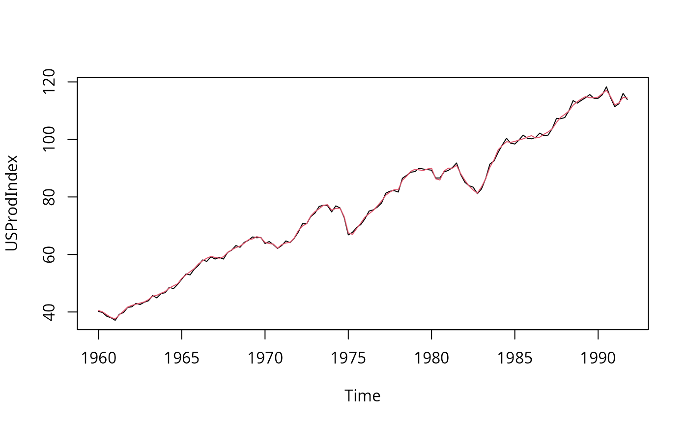
data("USProdIndex")
plot(USProdIndex, plot.type = "single", col = 1:2)


## EACF tables (Franses 1998, p. 99)
ctrafo <- function(x) residuals(lm(x ~ factor(cycle(x))))
ddiff <- function(x) diff(diff(x, frequency(x)), 1)
eacf <- function(y, lag = 12) {
  stopifnot(all(lag > 0))
  if(length(lag) < 2) lag <- 1:lag
  rval <- sapply(
    list(y = y, dy = diff(y), cdy = ctrafo(diff(y)),
         Dy = diff(y, frequency(y)), dDy = ddiff(y)),
    function(x) acf(x, plot = FALSE, lag.max = max(lag))$acf[lag + 1])
  rownames(rval) <- lag
  return(rval)
}

## Franses (1998), Table 5.1
round(eacf(log(USProdIndex[,1])), digits = 3)
#>        y     dy    cdy     Dy    dDy
#> 1  0.975  0.162  0.242  0.851  0.535
#> 2  0.947  0.140  0.196  0.586  0.162
#> 3  0.918 -0.110 -0.061  0.295 -0.051
#> 4  0.888  0.300  0.205  0.036 -0.328
#> 5  0.853 -0.268 -0.264 -0.126 -0.296
#> 6  0.821 -0.046 -0.032 -0.220 -0.190
#> 7  0.789 -0.249 -0.224 -0.274 -0.165
#> 8  0.761  0.120  0.008 -0.296 -0.204
#> 9  0.732 -0.257 -0.253 -0.262 -0.066
#> 10 0.705  0.015  0.044 -0.207  0.080
#> 11 0.676 -0.198 -0.165 -0.172  0.025
#> 12 0.649  0.199  0.099 -0.138  0.018

## Franses (1998), Equation 5.6: Unrestricted airline model
## (Franses: ma1 = 0.388 (0.063), ma4 = -0.739 (0.060), ma5 = -0.452 (0.069))
arima(log(USProdIndex[,1]), c(0, 1, 5), c(0, 1, 0), fixed = c(NA, 0, 0, NA, NA))
#> 
#> Call:
#> arima(x = log(USProdIndex[, 1]), order = c(0, 1, 5), seasonal = c(0, 1, 0), 
#>     fixed = c(NA, 0, 0, NA, NA))
#> 
#> Coefficients:
#>          ma1  ma2  ma3      ma4      ma5
#>       0.4603    0    0  -0.7731  -0.5313
#> s.e.  0.0707    0    0   0.0626   0.0713
#> 
#> sigma^2 estimated as 0.0003366:  log likelihood = 314.84,  aic = -621.69