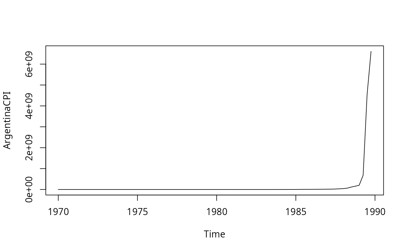
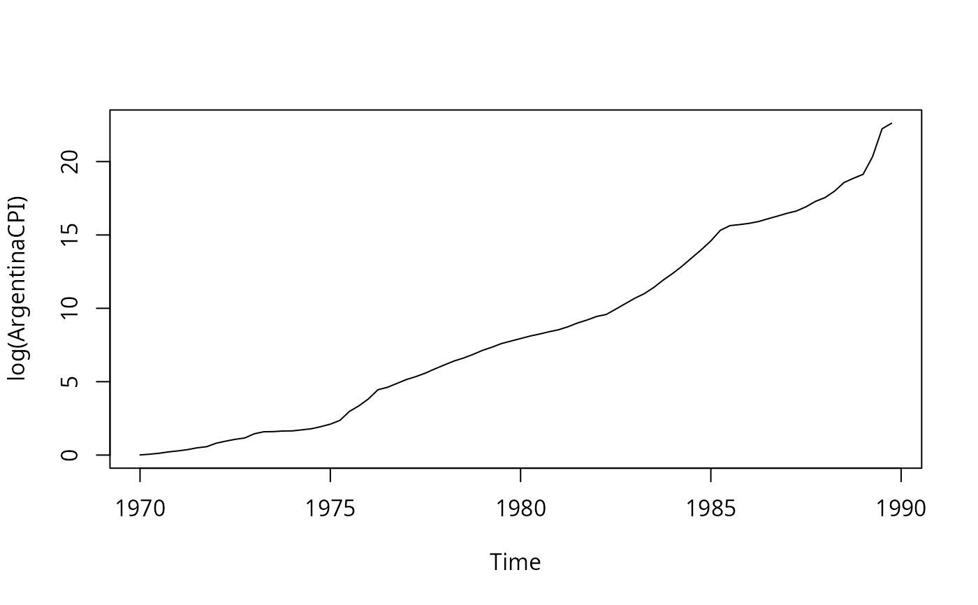
Consumer Price Index in Argentina

Time series of consumer price index (CPI) in Argentina (index with 1969(4) = 1).

Usage

data("ArgentinaCPI")

Format

A quarterly univariate time series from 1970(1) to 1989(4).

Source

Online complements to Franses (1998).

References

De Ruyter van Steveninck, M.A. (1996). The Impact of Capital Imports; Argentina 1970–1989. Amsterdam: Thesis Publishers.

Franses, P.H. (1998). Time Series Models for Business and Economic Forecasting. Cambridge, UK: Cambridge University Press.

See also

Franses1998

Examples

#> Loading required namespace: dynlm
data("ArgentinaCPI")
plot(ArgentinaCPI)

plot(log(ArgentinaCPI))


library("dynlm")
## estimation sample 1970.3-1988.4 means
acpi <- window(ArgentinaCPI, start = c(1970,1), end = c(1988,4)) 

## eq. (3.90), p.54
acpi_ols <- dynlm(d(log(acpi)) ~ L(d(log(acpi))))
summary(acpi_ols)
#> 
#> Time series regression with "ts" data:
#> Start = 1970(3), End = 1988(4)
#> 
#> Call:
#> dynlm(formula = d(log(acpi)) ~ L(d(log(acpi))))
#> 
#> Residuals:
#>      Min       1Q   Median       3Q      Max 
#> -0.35308 -0.05569 -0.01312  0.04952  0.35938 
#> 
#> Coefficients:
#>                 Estimate Std. Error t value Pr(>|t|)    
#> (Intercept)      0.07764    0.02458   3.158  0.00232 ** 
#> L(d(log(acpi)))  0.70359    0.08205   8.575 1.29e-12 ***
#> ---
#> Signif. codes:  0 ‘***’ 0.001 ‘**’ 0.01 ‘*’ 0.05 ‘.’ 0.1 ‘ ’ 1
#> 
#> Residual standard error: 0.1156 on 72 degrees of freedom
#> Multiple R-squared:  0.5053,	Adjusted R-squared:  0.4984 
#> F-statistic: 73.53 on 1 and 72 DF,  p-value: 1.293e-12
#> 

## alternatively
ar(diff(log(acpi)), order.max = 1, method = "ols") 
#> 
#> Call:
#> ar(x = diff(log(acpi)), order.max = 1, method = "ols")
#> 
#> Coefficients:
#>      1  
#> 0.7036  
#> 
#> Intercept: 0.003122 (0.01326) 
#> 
#> Order selected 1  sigma^2 estimated as  0.013