TV and Radio Advertising Expenditures Data

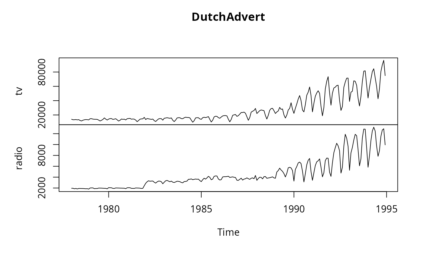
Time series of television and radio advertising expenditures (in real terms) in The Netherlands.

Usage

data("DutchAdvert")

Format

A four-weekly multiple time series from 1978(1) to 1994(13) with 2 variables.

tv: Television advertising expenditures.
radio: Radio advertising expenditures.

Source

Originally available as an online supplement to Franses (1998). Now available via online complements to Franses, van Dijk and Opschoor (2014).

https://www.cambridge.org/us/academic/subjects/economics/econometrics-statistics-and-mathematical-economics/time-series-models-business-and-economic-forecasting-2nd-edition

References

Franses, P.H. (1998). Time Series Models for Business and Economic Forecasting. Cambridge, UK: Cambridge University Press.

Franses, P.H., van Dijk, D. and Opschoor, A. (2014). Time Series Models for Business and Economic Forecasting, 2nd ed. Cambridge, UK: Cambridge University Press.

Examples

data("DutchAdvert")
plot(DutchAdvert)


## EACF tables (Franses 1998, Sec. 5.1, p. 99)
ctrafo <- function(x) residuals(lm(x ~ factor(cycle(x))))
ddiff <- function(x) diff(diff(x, frequency(x)), 1)
eacf <- function(y, lag = 12) {
  stopifnot(all(lag > 0))
  if(length(lag) < 2) lag <- 1:lag
  rval <- sapply(
    list(y = y, dy = diff(y), cdy = ctrafo(diff(y)),
         Dy = diff(y, frequency(y)), dDy = ddiff(y)),
    function(x) acf(x, plot = FALSE, lag.max = max(lag))$acf[lag + 1])
  rownames(rval) <- lag
  return(rval)
}

## Franses (1998, p. 103), Table 5.4
round(eacf(log(DutchAdvert[,"tv"]), lag = c(1:19, 26, 39)), digits = 3)
#>        y     dy    cdy    Dy    dDy
#> 1  0.933  0.215  0.039 0.663 -0.301
#> 2  0.836 -0.352 -0.255 0.529 -0.111
#> 3  0.781 -0.418 -0.316 0.471 -0.083
#> 4  0.774 -0.351 -0.301 0.466  0.044
#> 5  0.813 -0.013 -0.020 0.431  0.001
#> 6  0.857  0.417  0.346 0.393 -0.003
#> 7  0.848  0.438  0.409 0.357  0.036
#> 8  0.786 -0.008  0.024 0.299  0.008
#> 9  0.723 -0.348 -0.308 0.233 -0.031
#> 10 0.700 -0.398 -0.288 0.191 -0.022
#> 11 0.725 -0.324 -0.191 0.162  0.026
#> 12 0.788  0.240  0.109 0.119  0.105
#> 13 0.829  0.810  0.531 0.004 -0.412
#> 14 0.773  0.265  0.183 0.172  0.312
#> 15 0.683 -0.331 -0.210 0.125 -0.103
#> 16 0.630 -0.370 -0.222 0.146  0.096
#> 17 0.621 -0.334 -0.277 0.103  0.008
#> 18 0.656 -0.025 -0.053 0.050 -0.187
#> 19 0.699  0.383  0.274 0.127  0.003
#> 26 0.672  0.728  0.399 0.111 -0.002
#> 39 0.500  0.650  0.294 0.172  0.034