Black and White Pepper Prices
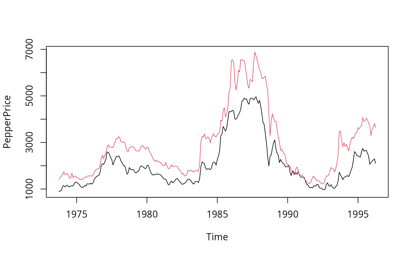
PepperPrice.RdTime series of average monthly European spot prices for black and white pepper (fair average quality) in US dollars per ton.
Usage
data("PepperPrice")Format
A monthly multiple time series from 1973(10) to 1996(4) with 2 variables.
- black
spot price for black pepper,
- white
spot price for white pepper.
Source
Originally available as an online supplement to Franses (1998). Now available via online complements to Franses, van Dijk and Opschoor (2014).
References
Franses, P.H. (1998). Time Series Models for Business and Economic Forecasting. Cambridge, UK: Cambridge University Press.
Franses, P.H., van Dijk, D. and Opschoor, A. (2014). Time Series Models for Business and Economic Forecasting, 2nd ed. Cambridge, UK: Cambridge University Press.
Examples
## data
data("PepperPrice", package = "AER")
plot(PepperPrice, plot.type = "single", col = 1:2)


## package
library("tseries")
library("urca")

## unit root tests
adf.test(log(PepperPrice[, "white"]))
#>
#> 	Augmented Dickey-Fuller Test
#>
#> data:  log(PepperPrice[, "white"])
#> Dickey-Fuller = -1.744, Lag order = 6, p-value = 0.6838
#> alternative hypothesis: stationary
#>
adf.test(diff(log(PepperPrice[, "white"])))
#> Warning: p-value smaller than printed p-value
#>
#> 	Augmented Dickey-Fuller Test
#>
#> data:  diff(log(PepperPrice[, "white"]))
#> Dickey-Fuller = -5.336, Lag order = 6, p-value = 0.01
#> alternative hypothesis: stationary
#>
pp.test(log(PepperPrice[, "white"]), type = "Z(t_alpha)")
#>
#> 	Phillips-Perron Unit Root Test
#>
#> data:  log(PepperPrice[, "white"])
#> Dickey-Fuller Z(t_alpha) = -1.6439, Truncation lag parameter = 5,
#> p-value = 0.726
#> alternative hypothesis: stationary
#>
pepper_ers <- ur.ers(log(PepperPrice[, "white"]),
  type = "DF-GLS", model = "const", lag.max = 4)
summary(pepper_ers)
#>
#> ###############################################
#> # Elliot, Rothenberg and Stock Unit Root Test #
#> ###############################################
#>
#> Test of type DF-GLS
#> detrending of series with intercept
#>
#>
#> Call:
#> lm(formula = dfgls.form, data = data.dfgls)
#>
#> Residuals:
#>      Min       1Q   Median       3Q      Max
#> -0.21135 -0.03069 -0.00108  0.03030  0.31018
#>
#> Coefficients:
#>               Estimate Std. Error t value Pr(>|t|)
#> yd.lag       -0.004022   0.006015  -0.669    0.504
#> yd.diff.lag1  0.336267   0.061986   5.425 1.32e-07 ***
#> yd.diff.lag2 -0.105024   0.065414  -1.606    0.110
#> yd.diff.lag3  0.001263   0.065366   0.019    0.985
#> yd.diff.lag4  0.011251   0.062085   0.181    0.856
#> ---
#> Signif. codes:  0 ‘***’ 0.001 ‘**’ 0.01 ‘*’ 0.05 ‘.’ 0.1 ‘ ’ 1
#>
#> Residual standard error: 0.06481 on 261 degrees of freedom
#> Multiple R-squared:  0.1028,	Adjusted R-squared:  0.0856
#> F-statistic:  5.98 on 5 and 261 DF,  p-value: 2.947e-05
#>
#>
#> Value of test-statistic is: -0.6686
#>
#> Critical values of DF-GLS are:
#>                  1pct  5pct 10pct
#> critical values -2.57 -1.94 -1.62
#>

## stationarity tests
kpss.test(log(PepperPrice[, "white"]))
#>
#> 	KPSS Test for Level Stationarity
#>
#> data:  log(PepperPrice[, "white"])
#> KPSS Level = 0.61733, Truncation lag parameter = 5, p-value = 0.02106
#>

## cointegration
po.test(log(PepperPrice))
#>
#> 	Phillips-Ouliaris Cointegration Test
#>
#> data:  log(PepperPrice)
#> Phillips-Ouliaris demeaned = -24.099, Truncation lag parameter = 2,
#> p-value = 0.02404
#>
pepper_jo <- ca.jo(log(PepperPrice), ecdet = "const", type = "trace")
summary(pepper_jo)
#>
#> ######################
#> # Johansen-Procedure #
#> ######################
#>
#> Test type: trace statistic , without linear trend and constant in cointegration
#>
#> Eigenvalues (lambda):
#> [1] 4.931953e-02 1.350807e-02 2.775558e-17
#>
#> Values of teststatistic and critical values of test:
#>
#>           test 10pct  5pct  1pct
#> r <= 1 |  3.66  7.52  9.24 12.97
#> r = 0  | 17.26 17.85 19.96 24.60
#>
#> Eigenvectors, normalised to first column:
#> (These are the cointegration relations)
#>
#>            black.l2 white.l2   constant
#> black.l2  1.0000000  1.00000   1.000000
#> white.l2 -0.8892307 -5.09942   2.280911
#> constant -0.5569943 33.02742 -20.032441
#>
#> Weights W:
#> (This is the loading matrix)
#>
#>            black.l2    white.l2      constant
#> black.d -0.07472300 0.002453210 -4.381722e-17
#> white.d  0.02015611 0.003537005  4.627140e-17
#>
pepper_jo2 <- ca.jo(log(PepperPrice), ecdet = "const", type = "eigen")
summary(pepper_jo2)
#>
#> ######################
#> # Johansen-Procedure #
#> ######################
#>
#> Test type: maximal eigenvalue statistic (lambda max) , without linear trend and constant in cointegration
#>
#> Eigenvalues (lambda):
#> [1] 4.931953e-02 1.350807e-02 2.775558e-17
#>
#> Values of teststatistic and critical values of test:
#>
#>           test 10pct  5pct  1pct
#> r <= 1 |  3.66  7.52  9.24 12.97
#> r = 0  | 13.61 13.75 15.67 20.20
#>
#> Eigenvectors, normalised to first column:
#> (These are the cointegration relations)
#>
#>            black.l2 white.l2   constant
#> black.l2  1.0000000  1.00000   1.000000
#> white.l2 -0.8892307 -5.09942   2.280911
#> constant -0.5569943 33.02742 -20.032441
#>
#> Weights W:
#> (This is the loading matrix)
#>
#>            black.l2    white.l2      constant
#> black.d -0.07472300 0.002453210 -4.381722e-17
#> white.d  0.02015611 0.003537005  4.627140e-17
#>
## package
library("tseries")
library("urca")
## unit root tests
adf.test(log(PepperPrice[, "white"]))
#>
#> Augmented Dickey-Fuller Test
#>
#> data: log(PepperPrice[, "white"])
#> Dickey-Fuller = -1.744, Lag order = 6, p-value = 0.6838
#> alternative hypothesis: stationary
#>
adf.test(diff(log(PepperPrice[, "white"])))
#> Warning: p-value smaller than printed p-value
#>
#> Augmented Dickey-Fuller Test
#>
#> data: diff(log(PepperPrice[, "white"]))
#> Dickey-Fuller = -5.336, Lag order = 6, p-value = 0.01
#> alternative hypothesis: stationary
#>
pp.test(log(PepperPrice[, "white"]), type = "Z(t_alpha)")
#>
#> Phillips-Perron Unit Root Test
#>
#> data: log(PepperPrice[, "white"])
#> Dickey-Fuller Z(t_alpha) = -1.6439, Truncation lag parameter = 5,
#> p-value = 0.726
#> alternative hypothesis: stationary
#>
pepper_ers <- ur.ers(log(PepperPrice[, "white"]),
type = "DF-GLS", model = "const", lag.max = 4)
summary(pepper_ers)
#>
#> ###############################################
#> # Elliot, Rothenberg and Stock Unit Root Test #
#> ###############################################
#>
#> Test of type DF-GLS
#> detrending of series with intercept
#>
#>
#> Call:
#> lm(formula = dfgls.form, data = data.dfgls)
#>
#> Residuals:
#> Min 1Q Median 3Q Max
#> -0.21135 -0.03069 -0.00108 0.03030 0.31018
#>
#> Coefficients:
#> Estimate Std. Error t value Pr(>|t|)
#> yd.lag -0.004022 0.006015 -0.669 0.504
#> yd.diff.lag1 0.336267 0.061986 5.425 1.32e-07 ***
#> yd.diff.lag2 -0.105024 0.065414 -1.606 0.110
#> yd.diff.lag3 0.001263 0.065366 0.019 0.985
#> yd.diff.lag4 0.011251 0.062085 0.181 0.856
#> ---
#> Signif. codes: 0 ‘***’ 0.001 ‘**’ 0.01 ‘*’ 0.05 ‘.’ 0.1 ‘ ’ 1
#>
#> Residual standard error: 0.06481 on 261 degrees of freedom
#> Multiple R-squared: 0.1028, Adjusted R-squared: 0.0856
#> F-statistic: 5.98 on 5 and 261 DF, p-value: 2.947e-05
#>
#>
#> Value of test-statistic is: -0.6686
#>
#> Critical values of DF-GLS are:
#> 1pct 5pct 10pct
#> critical values -2.57 -1.94 -1.62
#>
## stationarity tests
kpss.test(log(PepperPrice[, "white"]))
#>
#> KPSS Test for Level Stationarity
#>
#> data: log(PepperPrice[, "white"])
#> KPSS Level = 0.61733, Truncation lag parameter = 5, p-value = 0.02106
#>
## cointegration
po.test(log(PepperPrice))
#>
#> Phillips-Ouliaris Cointegration Test
#>
#> data: log(PepperPrice)
#> Phillips-Ouliaris demeaned = -24.099, Truncation lag parameter = 2,
#> p-value = 0.02404
#>
pepper_jo <- ca.jo(log(PepperPrice), ecdet = "const", type = "trace")
summary(pepper_jo)
#>
#> ######################
#> # Johansen-Procedure #
#> ######################
#>
#> Test type: trace statistic , without linear trend and constant in cointegration
#>
#> Eigenvalues (lambda):
#> [1] 4.931953e-02 1.350807e-02 2.775558e-17
#>
#> Values of teststatistic and critical values of test:
#>
#> test 10pct 5pct 1pct
#> r <= 1 | 3.66 7.52 9.24 12.97
#> r = 0 | 17.26 17.85 19.96 24.60
#>
#> Eigenvectors, normalised to first column:
#> (These are the cointegration relations)
#>
#> black.l2 white.l2 constant
#> black.l2 1.0000000 1.00000 1.000000
#> white.l2 -0.8892307 -5.09942 2.280911
#> constant -0.5569943 33.02742 -20.032441
#>
#> Weights W:
#> (This is the loading matrix)
#>
#> black.l2 white.l2 constant
#> black.d -0.07472300 0.002453210 -4.381722e-17
#> white.d 0.02015611 0.003537005 4.627140e-17
#>
pepper_jo2 <- ca.jo(log(PepperPrice), ecdet = "const", type = "eigen")
summary(pepper_jo2)
#>
#> ######################
#> # Johansen-Procedure #
#> ######################
#>
#> Test type: maximal eigenvalue statistic (lambda max) , without linear trend and constant in cointegration
#>
#> Eigenvalues (lambda):
#> [1] 4.931953e-02 1.350807e-02 2.775558e-17
#>
#> Values of teststatistic and critical values of test:
#>
#> test 10pct 5pct 1pct
#> r <= 1 | 3.66 7.52 9.24 12.97
#> r = 0 | 13.61 13.75 15.67 20.20
#>
#> Eigenvectors, normalised to first column:
#> (These are the cointegration relations)
#>
#> black.l2 white.l2 constant
#> black.l2 1.0000000 1.00000 1.000000
#> white.l2 -0.8892307 -5.09942 2.280911
#> constant -0.5569943 33.02742 -20.032441
#>
#> Weights W:
#> (This is the loading matrix)
#>
#> black.l2 white.l2 constant
#> black.d -0.07472300 0.002453210 -4.381722e-17
#> white.d 0.02015611 0.003537005 4.627140e-17
#>