Plot Estimated Systematical Bias with Confidence Bounds

This function plots the estimated systematical bias \(( Intercept + Slope * Refrencemethod ) - Referencemethod\) with confidence bounds, covering the whole range of reference method X or only part of it.

MCResult.plotBias(
  x,
  xn = 100,
  alpha = 0.05,
  add = FALSE,
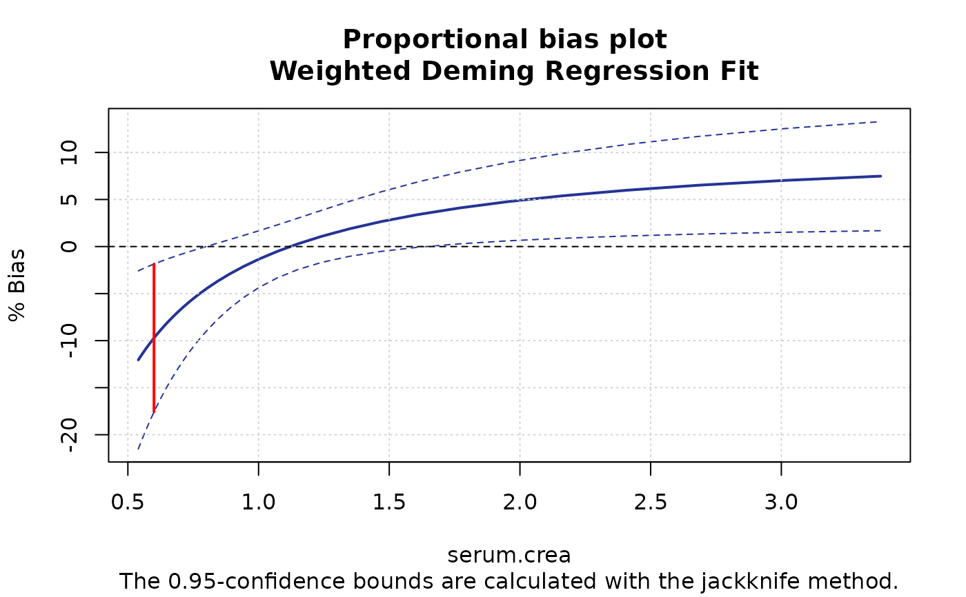
  prop = FALSE,
  xlim = NULL,
  ylim = NULL,
  bias = TRUE,
  bias.lty = 1,
  bias.lwd = 2,
  bias.col = NULL,
  ci.area = TRUE,
  ci.area.col = NULL,
  ci.border = FALSE,
  ci.border.col = NULL,
  ci.border.lwd = 1,
  ci.border.lty = 2,
  zeroline = TRUE,
  zeroline.col = NULL,
  zeroline.lty = 2,
  zeroline.lwd = 1,
  main = NULL,
  sub = NULL,
  add.grid = TRUE,
  xlab = NULL,
  ylab = NULL,
  cut.point = NULL,
  cut.point.col = "red",
  cut.point.lwd = 2,
  cut.point.lty = 1,
  ...
)

Arguments

x: object of class "MCResult".
xn: # number of poits for drawing of confidence bounds/area.
alpha: numeric value specifying the 100(1-alpha)% confidence level of confidence intervals (Default is 0.05).
add: logical value. If add=TRUE, the grafic will be drawn in current grafical window.
prop: a logical value. If prop=TRUE the proportional bias \( \%bias(Xc) = [ Intercept + (Slope-1) * Xc ] / Xc\) will be drawn.
xlim: limits of the x-axis. If xlim=NULL the x-limits will be calculated automatically.
ylim: limits of the y-axis. If ylim=NULL the y-limits will be calculated automatically.
bias: logical value. If identity=TRUE the bias line will be drawn. If ci.bounds=FALSE and ci.area=FALSE the bias line will be drawn always.
bias.lty: type of the bias line.
bias.lwd: width of the bias line.
bias.col: color of the bias line.
ci.area: logical value. If ci.area=TRUE (default) the confidence area will be drawn.
ci.area.col: color of the confidence area.
ci.border: logical value. If ci.border=TRUE the confidence limits will be drawn.
ci.border.col: color of the confidence limits.
ci.border.lwd: line width of confidence limits.
ci.border.lty: line type of confidence limits.
zeroline: logical value. If zeroline=TRUE the zero-line will be drawn.
zeroline.col: color of the zero-line.
zeroline.lty: type of the zero-line.
zeroline.lwd: width of the zero-line.
main: character string. The main title of plot. If main = NULL it will include regression name.
sub: character string. The subtitle of plot. If sub=NULL and ci.border=TRUE or ci.area=TRUE it will include the art of confidence bounds calculation.
add.grid: logical value. If grid=TRUE (default) the gridlines will be drawn.
xlab: label for the x-axis
ylab: label for the y-axis
cut.point: numeric value. Decision level of interest.
cut.point.col: color of the confidence bounds at the required decision level.
cut.point.lwd: line width of the confidence bounds at the required decision level.
cut.point.lty: line type of the confidence bounds at the required decision level.
...: further graphical parameters

Value

No return value, instead a plot is generated

Examples

#library("mcr")
data(creatinine,package="mcr")

creatinine <- creatinine[complete.cases(creatinine),]
x <- creatinine$serum.crea
y <- creatinine$plasma.crea

# Calculation of models
m1 <- mcreg(x,y,method.reg="WDeming", method.ci="jackknife",
                mref.name="serum.crea",mtest.name="plasma.crea", na.rm=TRUE)
#> Jackknife based calculation of standard error and confidence intervals according to Linnet's method.
m2 <- mcreg(x,y,method.reg="WDeming", method.ci="bootstrap",
                method.bootstrap.ci="BCa",mref.name="serum.crea",
                mtest.name="plasma.crea", na.rm=TRUE)
#> The global.sigma is calculated with Linnet's method

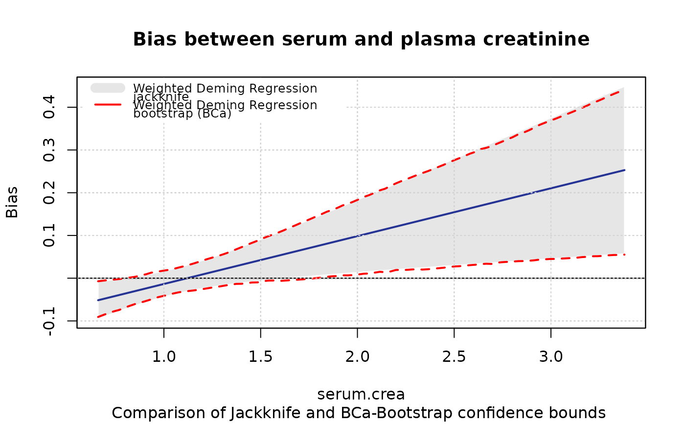
# Grafical comparison of systematical Bias of two models
plotBias(m1, zeroline=TRUE,zeroline.col="black",zeroline.lty=1,
                ci.area=TRUE,ci.border=FALSE, ci.area.col=grey(0.9),
                main = "Bias between serum and plasma creatinine",
                sub="Comparison of Jackknife and BCa-Bootstrap confidence bounds ")
plotBias(m2, ci.area=FALSE, ci.border=TRUE, ci.border.lwd=2,
                ci.border.col="red",bias=FALSE ,add=TRUE)
includeLegend(place="topleft",models=list(m1,m2), lwd=c(10,2),
                lty=c(2,1),colors=c(grey(0.9),"red"), bias=TRUE,
                design="1", digits=4)


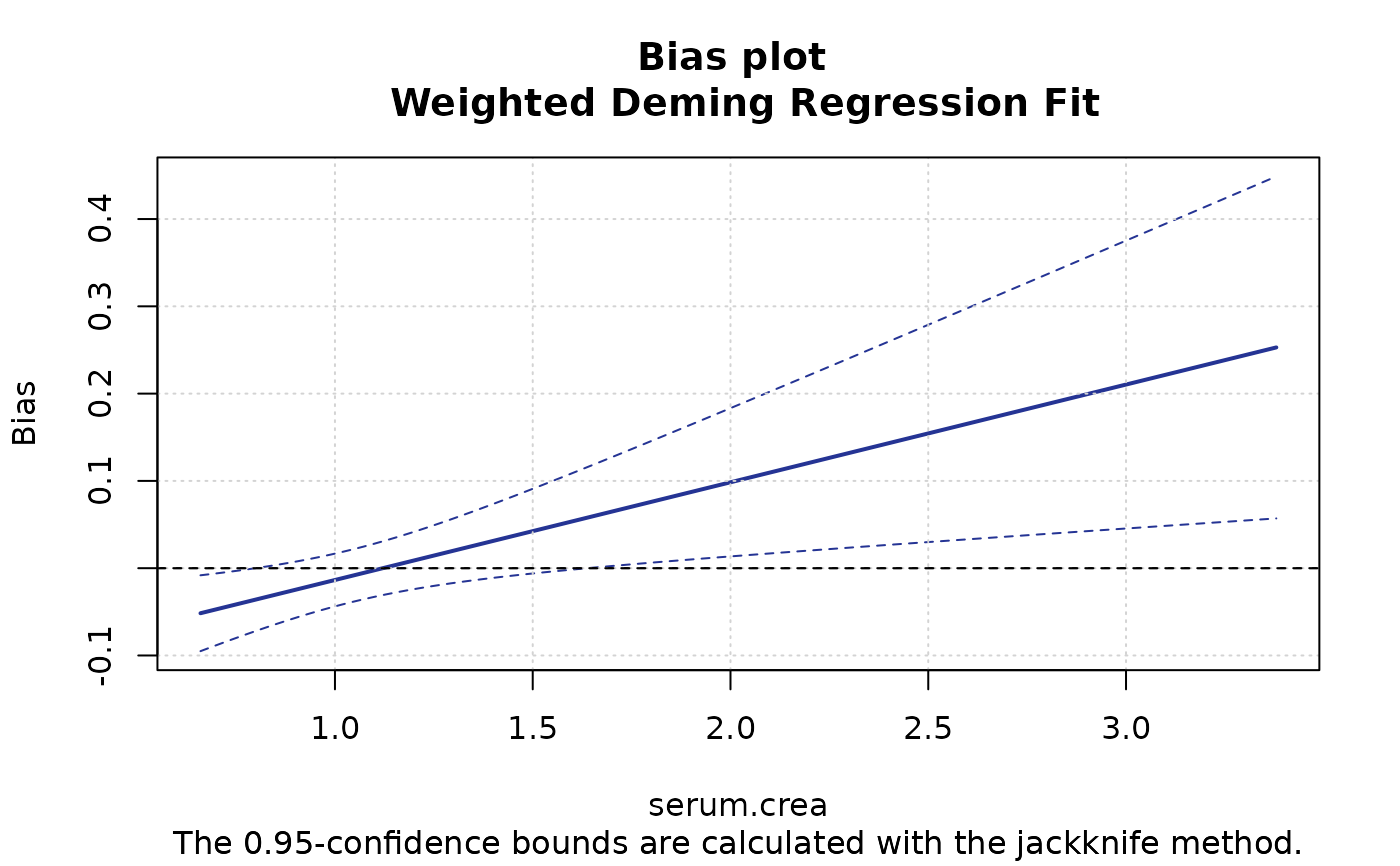
# Drawing of proportional bias
plotBias(m1, ci.area=FALSE, ci.border=TRUE)

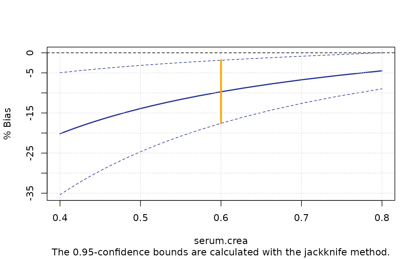
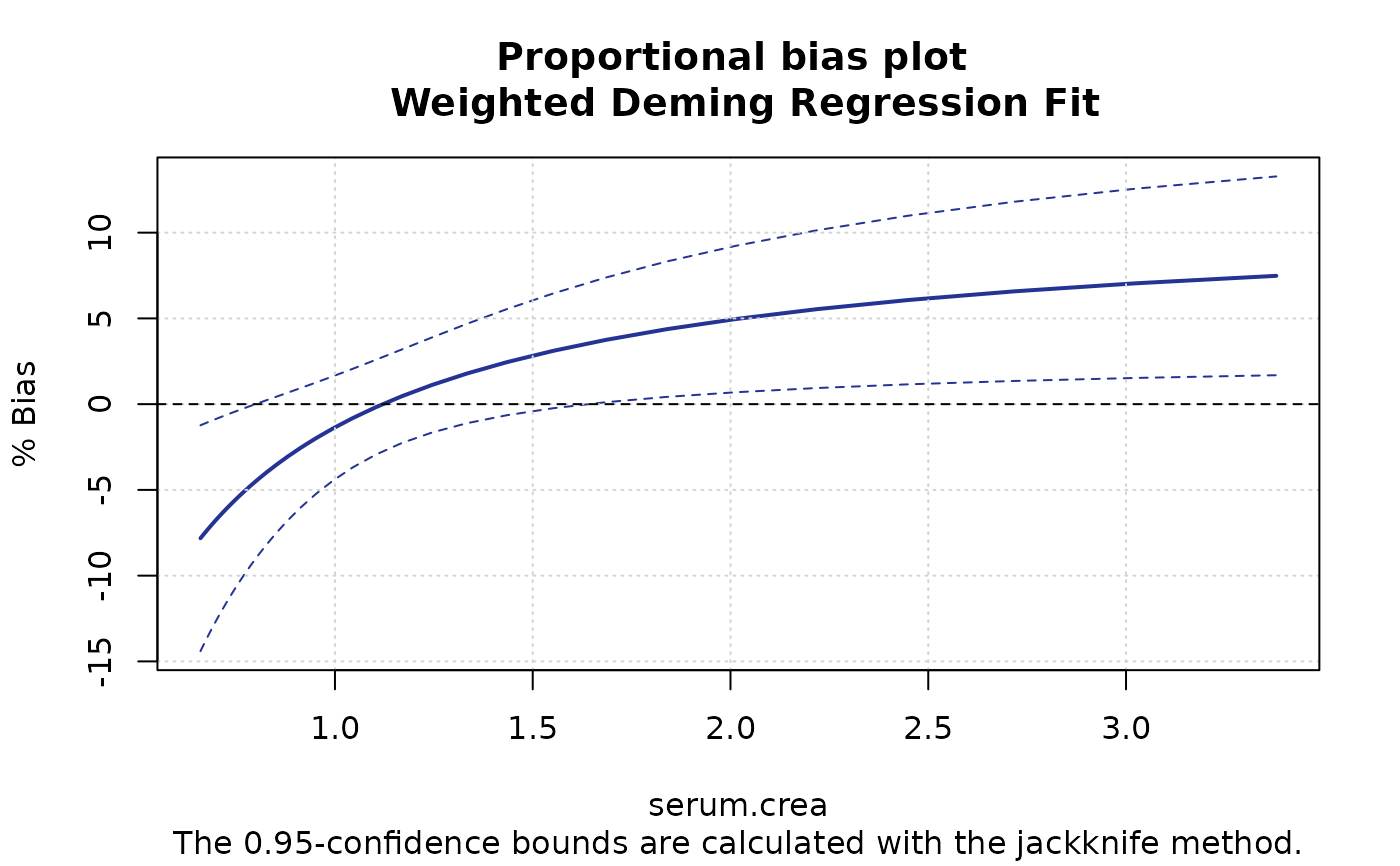
plotBias(m1, ci.area=FALSE, ci.border=TRUE, prop=TRUE)

plotBias(m1, ci.area=FALSE, ci.border=TRUE, prop=TRUE, cut.point=0.6)

plotBias(m1, ci.area=FALSE, ci.border=TRUE, prop=TRUE, cut.point=0.6,
             xlim=c(0.4,0.8),cut.point.col="orange", cut.point.lwd=3, main ="")

Plot Estimated Systematical Bias with Confidence Bounds

Arguments

Value

See also

Examples