Scatterplot Matrices

This function provides a convenient interface to the pairs function to produce enhanced scatterplot matrices, including univariate displays on the diagonal and a variety of fitted lines, smoothers, variance functions, and concentration ellipsoids. spm is an abbreviation for scatterplotMatrix.

Usage

scatterplotMatrix(x, ...)

# S3 method for class 'formula'
scatterplotMatrix(formula, data=NULL, subset, ...)

# Default S3 method
scatterplotMatrix(x, smooth = TRUE,
    id = FALSE, legend = TRUE, regLine = TRUE,
    ellipse = FALSE, var.labels = colnames(x), diagonal = TRUE,
    plot.points = TRUE, groups = NULL, by.groups = TRUE,
    use = c("complete.obs", "pairwise.complete.obs"), col =
    carPalette()[-1], pch = 1:n.groups, cex = par("cex"),
    cex.axis = par("cex.axis"), cex.labels = NULL,
    cex.main = par("cex.main"), row1attop = TRUE, ...)

spm(x, ...)

Arguments

x: a data matrix or a numeric data frame.
formula: a one-sided “model” formula, of the form ~ x1 + x2 + ... + xk or ~ x1 + x2 + ... + xk | z where z evaluates to a factor or other variable to divide the data into groups.
data: for scatterplotMatrix.formula, a data frame within which to evaluate the formula.
subset: expression defining a subset of observations.
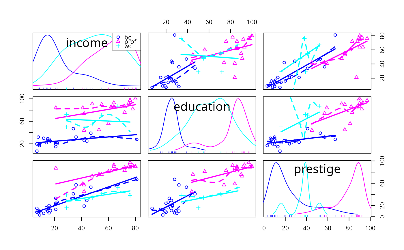
smooth: specifies a nonparametric estimate of the mean or median function of the vertical axis variable given the horizontal axis variable and optionally a nonparametric estimate of the spread or variance function. If smooth=FALSE neither function is drawn. If smooth=TRUE, then both the mean function and variance funtions are drawn for ungrouped data, and the mean function only is drawn for grouped data. The default smoother is loessLine, which uses the loess function from the stats package. This smoother is fast and reliable. See the details below for changing the smoother, line type, width and color, of the added lines, and adding arguments for the smoother.
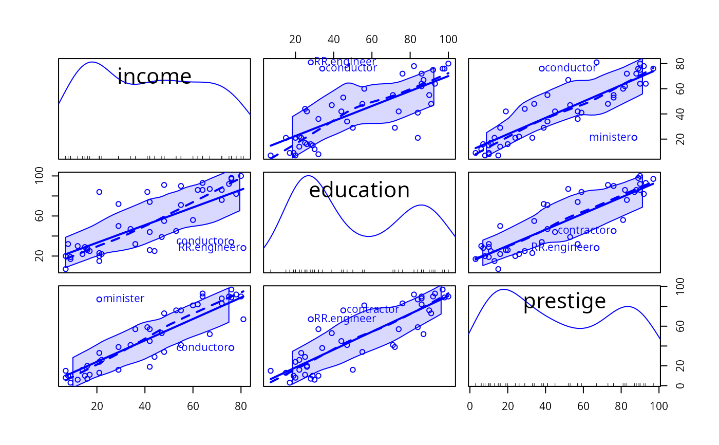
id: controls point identification; if FALSE (the default), no points are identified; can be a list of named arguments to the showLabels function; TRUE is equivalent to list(method="mahal", n=2, cex=1, location="lr"), which identifies the 2 points (in each group, if by.groups=TRUE) with the largest Mahalanobis distances from the center of the data; list(method="identify") for interactive point identification is not allowed.
legend: controls placement, point size, and text size of a legend if the plot is drawn by groups; if FALSE, the legend is suppressed. Can be a list with the named element coords specifying the position of the legend in any form acceptable to the legend function, and elements pt.cex and cex corresponding respectively to the pt.cex and cex arguments of the legend function; TRUE (the default) is equivalent to list(coords=NULL, pt.cex=cex, cex=cex), for which placement will vary by the the value of the diagonal argument—e.g., "topright" for diagonal=TRUE.
regLine: controls adding a fitted regression line to each plot, or to each group of points if by.groups=TRUE. If regLine=FALSE, no line is drawn. This argument can also be a list with named list, with default regLine=TRUE equivalent to regLine = list(method=lm, lty=1, lwd=2, col=col[1]) specifying the name of the function that computes the line, with line type 1 (solid) of relative line width 2 and the color equal to the first value in the argument col. Setting method=MASS::rlm would fit using a robust regression.
ellipse: controls plotting data-concentration ellipses. If FALSE (the default), no ellipses are plotted. Can be a list of named values giving levels, a vector of one or more bivariate-normal probability-contour levels at which to plot the ellipses; robust, a logical value determing whether to use the cov.trob function in the MASS package to calculate the center and covariance matrix for the data ellipses; and fill and fill.alpha, which control whether the ellipse is filled and the transparency of the fill. TRUE is equivalent to list(levels=c(.5, .95), robust=TRUE, fill=TRUE, fill.alpha=0.2).
var.labels: variable labels (for the diagonal of the plot).
diagonal: contents of the diagonal panels of the plot. If diagonal=TRUE adaptive kernel density estimates are plotted, separately for each group if grouping is present. diagonal=FALSE suppresses the diagonal entries. See details below for other choices for the diagonal.
plot.points: if TRUE the points are plotted in each off-diagonal panel.
groups: a factor or other variable dividing the data into groups; groups are plotted with different colors and plotting characters.
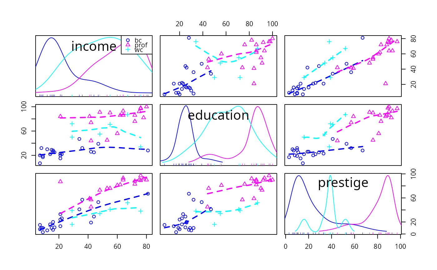
by.groups: if TRUE, the default, regression lines and smooths are fit by groups.
use: if "complete.obs" (the default), cases with missing data are omitted; if "pairwise.complete.obs"), all valid cases are used in each panel of the plot.
pch: plotting characters for points; default is the plotting characters in order (see par).
col: colors for points; the default is carPalette starting at the second color. The color of the regLine and smooth are the same as for points but can be changed using the the regLine and smooth arguments.
cex: relative size of plotted points. You can use cex = 0.001 to suppress the plotting of points if all you want to show are other graphical features, such as data ellipses, regression lines, smooths, etc.
cex.axis: relative size of axis labels
cex.labels: relative size of labels on the diagonal
cex.main: relative size of the main title, if any
row1attop: If TRUE (the default) the first row is at the top, as in a matrix, as opposed to at the bottom, as in graph (argument suggested by Richard Heiberger).
...: arguments to pass down.

Details

Many arguments to scatterplotMatrix were changed in version 3 of car, to simplify use of this function.

The smooth argument is usually either set to TRUE or FALSE to draw, or omit, the smoother. Alternatively smooth can be set to a list of arguments. The default behavior of smooth=TRUE is equivalent to smooth=list(smoother=loessLine, spread=TRUE, lty.smooth=1, lwd.smooth=1.5, lty.spread=3, lwd.spread=1), specifying the smoother to be used, including the spread or variance smooth, and the line widths and types for the curves. You can also specify the colors you want to use for the mean and variance smooths with the arguments col.smooth and col.spread. Alternative smoothers are gamline which uses the gam function from the mgcv package, and quantregLine which uses quantile regression to estimate the median and quartile functions using rqss from the quantreg package. All of these smoothers have one or more arguments described on their help pages, and these arguments can be added to the smooth argument; for example, smooth = list(span=1/2) would use the default loessLine smoother, include the variance smooth, and change the value of the smoothing parameter to 1/2. For loessLine and gamLine the variance smooth is estimated by separately smoothing the squared positive and negative residuals from the mean smooth, using the same type of smoother. The displayed curves are equal to the mean smooth plus the square root of the fit to the positive squared residuals, and the mean fit minus the square root of the smooth of the negative squared residuals. The lines therefore represent the comnditional variabiliity at each value on the horizontal axis. Because smoothing is done separately for positive and negative residuals, the variation shown will generally not be symmetric about the fitted mean function. For the quantregLine method, the center estimates the median for each value on the horizontal axis, and the spread estimates the lower and upper quartiles of the estimated conditional distribution for each value of the horizontal axis.

The sub-arguments spread, lty.spread and col.spread of the smooth argument are equivalent to the newer var, col.var and lty.var, respectively, recognizing that the spread is a measuure of conditional variability.

By default the diagonal argument is used to draw kernel density estimates of the variables by setting diagonal=TRUE, which is equivalent to setting diagonal = list(method="adaptiveDensity", bw=bw.nrd0, adjust=1, kernel=dnorm, na.rm=TRUE). The additional arguments shown are descibed at adaptiveKernel. The other methods avaliable, with their default arguments, are diagonal=list(method="density", bw="nrd0", adjust=1, kernel="gaussian", na.rm=TRUE) which uses density for nonadaptive kernel density estimation; diagonal=list(method ="histogram", breaks="FD") which uses hist for drawing a histogram that ignores grouping, if present; diagonal=list(method="boxplot") with no additional arguments which draws (parallel) boxplots; diagonal=list(method="qqplot") with no additional arguments which draws a normal QQ plot; and diagonal=list(method="oned") with no additional arguments which draws a rug plot tilted to the diagonal, as suggested by Richard Heiberger.

Earlier versions of scatterplotMatrix included arguments transform and family to estimate power transformations using the powerTransform function before drawing the plot. The same functionality can be achieved by calling powerTransform directly to estimate a transformation, saving the transformed variables, and then plotting.

Value

NULL, returned invisibly. This function is used for its side effect: producing a plot. If point identification is used, a vector of identified points is returned.

Author

John Fox jfox@mcmaster.ca

References

Fox, J. and Weisberg, S. (2019) An R Companion to Applied Regression, Third Edition, Sage.

Examples

scatterplotMatrix(~ income + education + prestige | type, data=Duncan)

scatterplotMatrix(~ income + education + prestige | type, data=Duncan,
    regLine=FALSE, smooth=list(span=1))

scatterplotMatrix(~ income + education + prestige,
    data=Duncan, id=TRUE, smooth=list(method=gamLine))