Nonparametric Density Estimates

densityPlot contructs and graphs nonparametric density estimates, possibly conditioned on a factor, using the standard R density function or by default adaptiveKernel, which computes an adaptive kernel density estimate. depan provides the Epanechnikov kernel and dbiwt provides the biweight kernel.

Usage

densityPlot(x, ...)

# Default S3 method
densityPlot(x, g, method=c("adaptive", "kernel"),
    bw=if (method == "adaptive") bw.nrd0 else "SJ", adjust=1,
    kernel, xlim, ylim,
    normalize=FALSE, xlab=deparse(substitute(x)), ylab="Density", main="",
    col=carPalette(), lty=seq_along(col), lwd=2, grid=TRUE,
    legend=TRUE, show.bw=FALSE, rug=TRUE, ...)

# S3 method for class 'formula'
densityPlot(formula, data=NULL, subset,
    na.action=NULL, xlab, ylab, main="", legend=TRUE, ...)

adaptiveKernel(x, kernel=dnorm, bw=bw.nrd0, adjust=1.0, n=500,
    from, to, cut=3, na.rm=TRUE)
    
depan(x)
dbiwt(x)

Arguments

x: a numeric variable, the density of which is estimated; for depan and dbiwt, the argument of the kernel function.
g: an optional factor to divide the data.
formula: an R model formula, of the form ~ variable to estimate the unconditional density of variable, or variable ~ factor to estimate the density of variable within each level of factor.
data: an optional data frame containing the data.
subset: an optional vector defining a subset of the data.
na.action: a function to handle missing values; defaults to the value of the R na.action option, initially set to na.omit.
method: either "adaptive" (the default) for an adaptive-kernel estimate or "kernel" for a fixed-bandwidth kernel estimate.
bw: the geometric mean bandwidth for the adaptive-kernel or bandwidth of the kernel density estimate(s). Must be a numerical value or a function to compute the bandwidth (default bw.nrd0) for the adaptive kernel estimate; for the kernel estimate, may either the quoted name of a rule to compute the bandwidth, or a numeric value. If plotting by groups, bw may be a vector of values, one for each group. See density and bw.SJ for details of the kernel estimator.
adjust: a multiplicative adjustment factor for the bandwidth; the default, 1, indicates no adjustment; if plotting by groups, adjust may be a vector of adjustment factors, one for each group. The default bandwidth-selection rule tends to give a value that's too large if the distribution is asymmetric or has multiple modes; try setting adjust < 1, particularly for the adaptive-kernel estimator.
kernel: for densityPlot this is the name of the kernel function for the kernel estimator (the default is "gaussian", see density); or a kernel function for the adaptive-kernel estimator (the default is dnorm, producing the Gaussian kernel). For adaptivekernel this is a kernel function, defaulting to dnorm, which is the Gaussian kernel (standard-normal density).
xlim, ylim: axis limits; if missing, determined from the range of x-values at which the densities are estimated and the estimated densities.
normalize: if TRUE (the default is FALSE), the estimated densities are rescaled to integrate approximately to 1; particularly useful if the density is estimated over a restricted domain, as when from or to are specified.
xlab: label for the horizontal-axis; defaults to the name of the variable x.
ylab: label for the vertical axis; defaults to "Density".
main: plot title; default is empty.
col: vector of colors for the density estimate(s); defaults to the color carPalette.
lty: vector of line types for the density estimate(s); defaults to the successive integers, starting at 1.
lwd: line width for the density estimate(s); defaults to 2.
grid: if TRUE (the default), grid lines are drawn on the plot.
legend: a list of up to two named elements: location, for the legend when densities are plotted for several groups, defaults to "upperright" (see legend); and title of the legend, which defaults to the name of the grouping factor. If TRUE, the default, the default values are used; if FALSE, the legend is suppressed.
n: number of equally spaced points at which the adaptive-kernel estimator is evaluated; the default is 500.
from, to, cut: the range over which the density estimate is computed; the default, if missing, is min(x) - cut*bw, max(x) + cut*bw.
na.rm: remove missing values from x in computing the adaptive-kernel estimate? The default is TRUE.
show.bw: if TRUE, show the bandwidth(s) in the horizontal-axis label or (for multiple groups) the legend; the default is FALSE.
rug: if TRUE (the default), draw a rug plot (one-dimentional scatterplot) at the bottom of the density estimate.
...: arguments to be passed down to graphics functions.

Details

If you use a different kernel function than the default dnorm that has a standard deviation different from 1 along with an automatic rule like the default function bw.nrd0, you can attach an attribute to the kernel function named "scale" that gives its standard deviation. This is true for the two supplied kernels, depan and dbiwt

Value

densityPlot invisibly returns the "density" object computed (or list of "density" objects) and draws a graph. adaptiveKernel returns an object of class "density" (see density).

References

Fox, J. and Weisberg, S. (2019) An R Companion to Applied Regression, Third Edition, Sage.

W. N. Venables and B. D. Ripley (2002) Modern Applied Statistics with S. New York: Springer.

B.W. Silverman (1986) Density Estimation for Statistics and Data Analysis. London: Chapman and Hall.

Author

John Fox jfox@mcmaster.ca

Examples

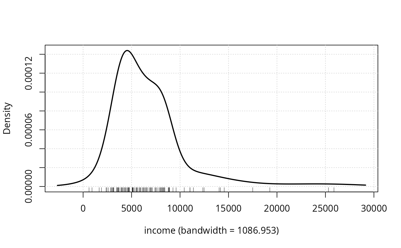
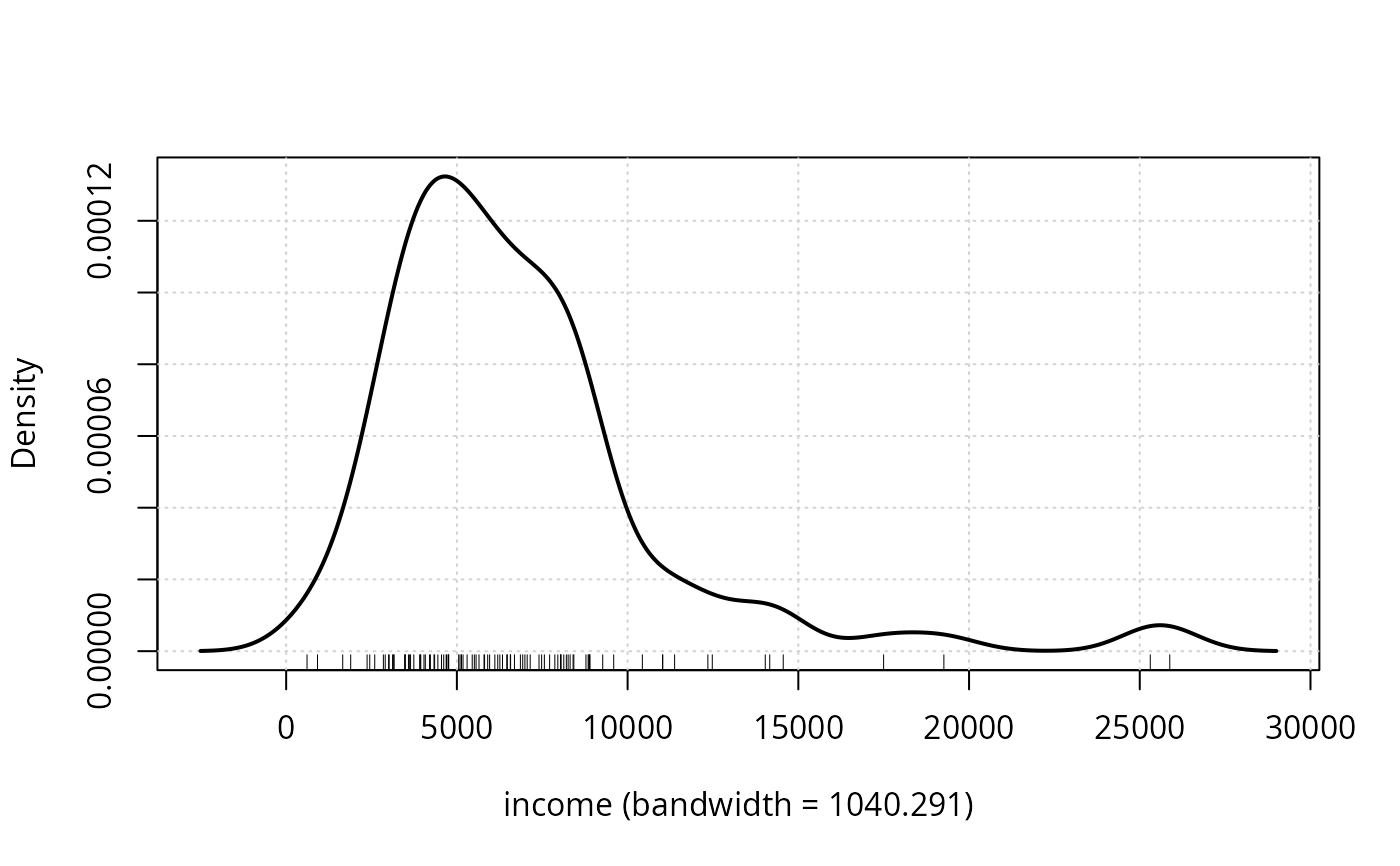
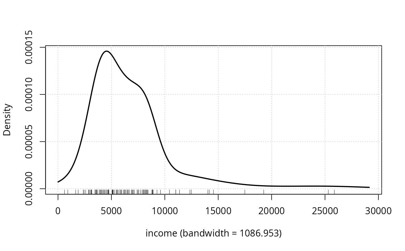
densityPlot(~ income, show.bw=TRUE, method="kernel", data=Prestige)

densityPlot(~ income, show.bw=TRUE, data=Prestige)

densityPlot(~ income, from=0, normalize=TRUE, show.bw=TRUE, data=Prestige)


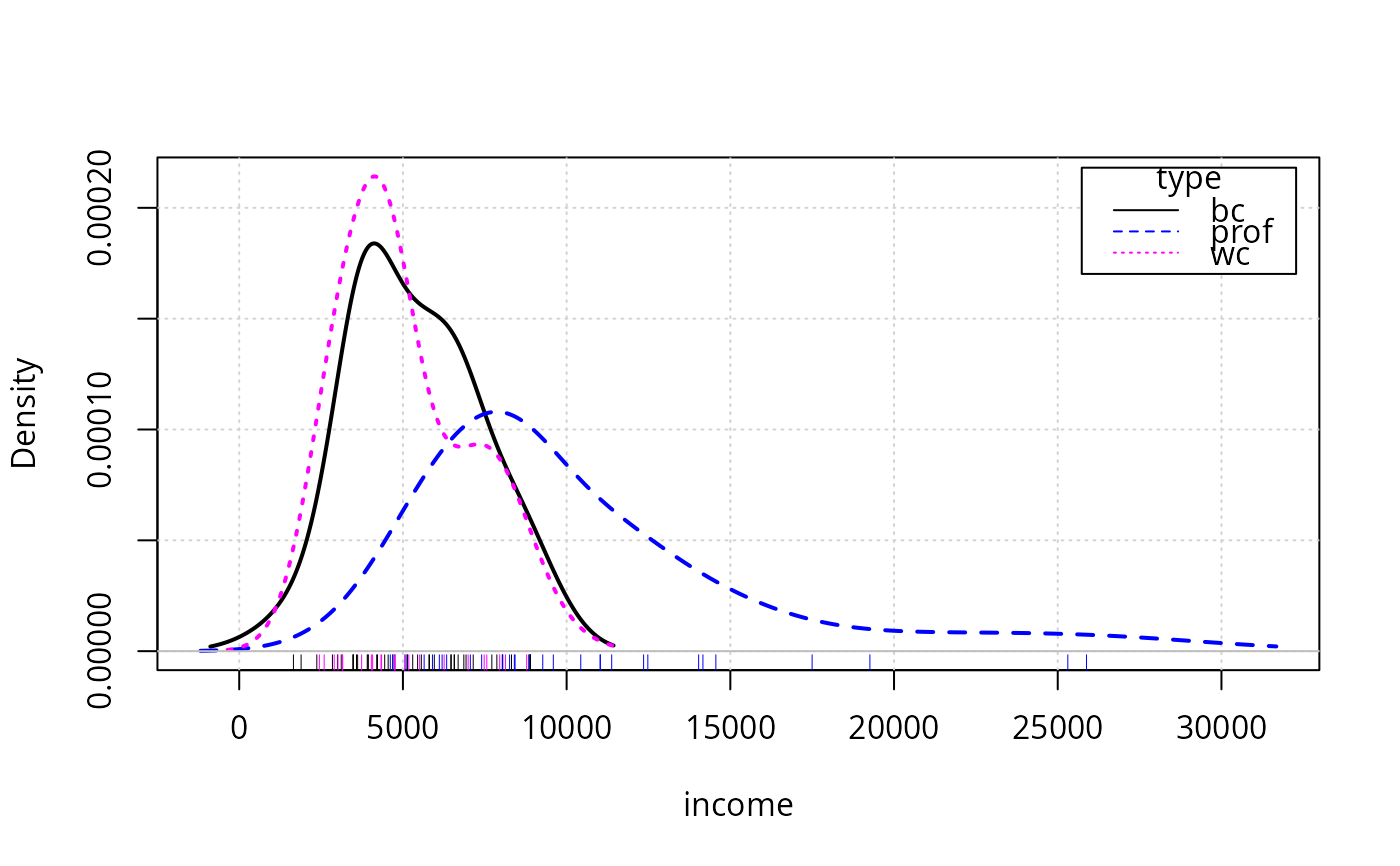
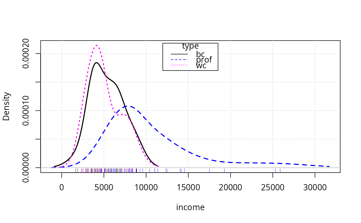
densityPlot(income ~ type, data=Prestige)

densityPlot(~ income, show.bw=TRUE, method="kernel", data=Prestige)

densityPlot(~ income, show.bw=TRUE, data=Prestige)

densityPlot(~ income, from=0, normalize=TRUE, show.bw=TRUE, data=Prestige)


densityPlot(income ~ type, kernel=depan, data=Prestige)

densityPlot(income ~ type, kernel=depan, legend=list(location="top"), data=Prestige)


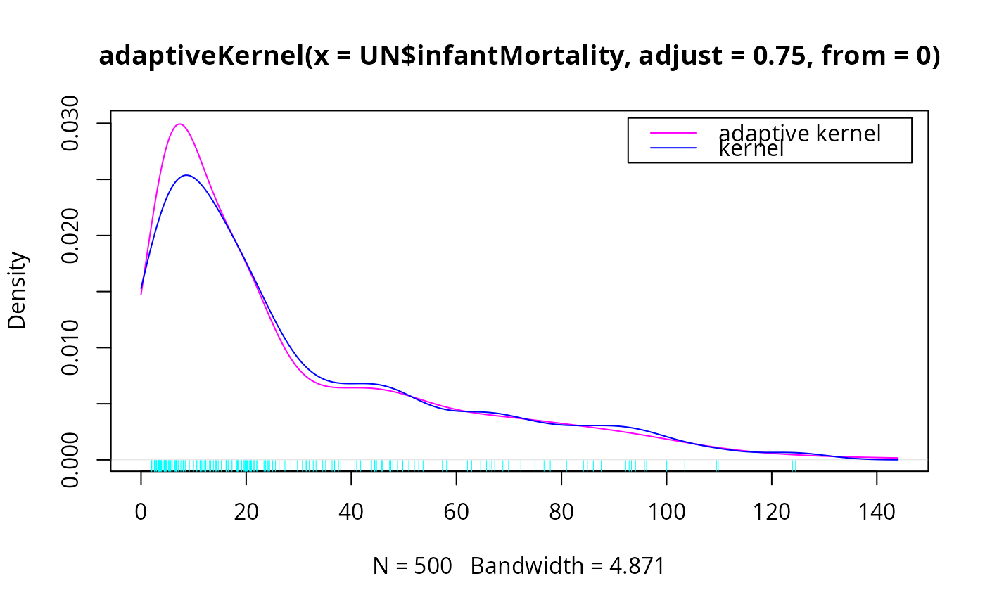
plot(adaptiveKernel(UN$infantMortality, from=0, adjust=0.75), col="magenta")
lines(density(na.omit(UN$infantMortality), from=0, adjust=0.75), col="blue")
rug(UN$infantMortality, col="cyan")
legend("topright", col=c("magenta", "blue"), lty=1,
       legend=c("adaptive kernel", "kernel"), inset=0.02)



plot(adaptiveKernel(UN$infantMortality, from=0, adjust=0.75), col="magenta")
lines(density(na.omit(UN$infantMortality), from=0, adjust=0.75), col="blue")
rug(UN$infantMortality, col="cyan")
legend("topright", col=c("magenta", "blue"), lty=1,
       legend=c("adaptive kernel", "kernel"), inset=0.02)