Enhanced Scatterplots with Marginal Boxplots, Point Marking, Smoothers, and More
scatterplot.RdThis function uses basic R graphics to draw a two-dimensional scatterplot, with options to allow for plot enhancements that are often helpful with regression problems. Enhancements include adding marginal boxplots, estimated mean and variance functions using either parametric or nonparametric methods, point identification, jittering, setting characteristics of points and lines like color, size and symbol, marking points and fitting lines conditional on a grouping variable, and other enhancements.
sp is an abbreviation for scatterplot.
Usage
scatterplot(x, ...)

# S3 method for class 'formula'
scatterplot(formula, data, subset, xlab, ylab, id=FALSE,
    legend=TRUE, ...)

# Default S3 method
scatterplot(x, y, boxplots=if (by.groups) "" else "xy",
        regLine=TRUE, legend=TRUE, id=FALSE, ellipse=FALSE, grid=TRUE,
        smooth=TRUE,
        groups, by.groups=!missing(groups),
        xlab=deparse(substitute(x)), ylab=deparse(substitute(y)),
        log="", jitter=list(), cex=par("cex"),
        col=carPalette()[-1], pch=1:n.groups,
        reset.par=TRUE, ...)

sp(x, ...)
Arguments
- x
vector of horizontal coordinates (or first argument of generic function).
- y
vector of vertical coordinates.
- formula
a model formula, of the form
y ~ xor, if plotting by groups,y ~ x | z, wherezevaluates to a factor or other variable dividing the data into groups. Ifxis a factor, then parallel boxplots are produced using theBoxplotfunction.- data
data frame within which to evaluate the formula.
- subset
expression defining a subset of observations.
- boxplots
if
"x"a marginal boxplot for the horizontalx-axis is drawn below the plot; if"y"a marginal boxplot for verticaly-axis is drawn to the left of the plot; if"xy"both marginal boxplots are drawn; set to""orFALSEto suppress both boxplots.- regLine
controls adding a fitted regression line to the plot. if
regLine=FALSE, no line is drawn. IfTRUE, the default, an OLS line is fit. This argument can also be a list. The default ofTRUEis equivalent toregLine=list(method=lm, lty=1, lwd=2, col=col), which specifies using thelmfunction to estimate the fitted line, to draw a solid line (lty=1) of width 2 times the nominal width (lwd=2) in the color given by the first element of thecolargument described below.- legend
when the plot is drawn by groups and
legend=TRUE, controls placement and properties of a legend; ifFALSE, the legend is suppressed. Can be a list of named arguments, as follows:titlefor the legend;inset, giving space as a proportion of the axes to offset the legend from the axes;coordsspecifying the position of the legend in any form acceptable to thelegendfunction or, if not given, the legend is placed above the plot in the upper margin;columnsfor the legend, determined automatically to prefer a horizontal layout if not given explicitly;cexgiving the relative size of the legend symbols and text.TRUE(the default) is equivalent tolist(title=deparse(substitute(groups)), inset=0.02, cex=1).- id
controls point identification; if
FALSE(the default), no points are identified; can be a list of named arguments to theshowLabelsfunction;TRUEis equivalent tolist(method="mahal", n=2, cex=1, col=carPalette()[-1], location="lr"), which identifies the 2 points (in each group) with the largest Mahalanobis distances from the center of the data. SeeshowLabelsfor a description of the other arguments. The default behavior ofidis not the same in all graphics functions in car, as themethodused depends on the type of plot.- ellipse
controls plotting data-concentration ellipses. If
FALSE(the default), no ellipses are plotted. Can be a list of named values givinglevels, a vector of one or more bivariate-normal probability-contour levels at which to plot the ellipses;robust, a logical value determing whether to use thecov.trobfunction in the MASS package to calculate the center and covariance matrix for the data ellipses; andfillandfill.alpha, which control whether the ellipse is filled and the transparency of the fill.TRUEis equivalent tolist(levels=c(.5, .95), robust=TRUE, fill=TRUE, fill.alpha=0.2).- grid
If TRUE, the default, a light-gray background grid is put on the graph
- smooth
specifies a nonparametric estimate of the mean or median function of the vertical axis variable given the horizontal axis variable and optionally a nonparametric estimate of the conditional variance. If
smooth=FALSEneither function is drawn. Ifsmooth=TRUE, then both the mean function and variance funtions are drawn for ungrouped data, and the mean function only is drawn for grouped data. The default smoother isloessLine, which uses theloessfunction from the stats package. This smoother is fast and reliable. See the details below for changing the smoother, line type, width and color, of the added lines, and adding arguments for the smoother.- groups
a factor or other variable dividing the data into groups; groups are plotted with different colors, plotting characters, fits, and smooths. Using this argument is equivalent to specifying the grouping variable in the formula.
- by.groups
if
TRUE(the default when there are groups), regression lines are fit by groups.- xlab
label for horizontal axis.
- ylab
label for vertical axis.
- log
same as the
logargument toplot, to produce log axes.- jitter
a list with elements
xoryor both, specifying jitter factors for the horizontal and vertical coordinates of the points in the scatterplot. Thejitterfunction is used to randomly perturb the points; specifying a factor of1produces the default jitter. Fitted lines are unaffected by the jitter.- col
with no grouping, this specifies a color for plotted points; with grouping, this argument should be a vector of colors of length at least equal to the number of groups. The default is value returned by
carPalette[-1].- pch
plotting characters for points; default is the plotting characters in order (see
par).- cex
sets the size of plotting characters, with
cex=1the standard size. You can usecex = 0to suppress the plotting of points if all you want to show are other graphical features, such as data ellipses, regression lines, smooths, etc. You can also set the sizes of other elements with the argumentscex.axis,cex.lab,cex.main, andcex.sub. Seepar.- reset.par
if
TRUE(the default) then plotting parameters are reset to their previous values whenscatterplotexits; ifFALSEthen themarandmfcolparameters are altered for the current plotting device. Set toFALSEif you want to add graphical elements (such as lines) to the plot.- ...
other arguments passed down and to
plot. For example, the argumentlassets the style of the axis labels, andxlimandylimset the limits on the horizontal and vertical axes, respectively; seepar.
Details
Many arguments to scatterplot were changed in version 3 of car to simplify use of this function.
The smooth argument is used to control adding smooth curves to the plot to estimate the conditional center of the vertical axis variable given the horizontal axis variable, and also the conditional variability. Setting smooth=FALSE omits all smoothers, while smooth=TRUE, the default, includes default smoothers. Alternatively smooth can be set to a list of subarguments that provide finer control over the smoothing.
The default behavior of smooth=TRUE is equivalent to smooth=list(smoother=loessLine, var=!by.groups, lty.var=2, lty.var=4, style="filled", alpha=0.15, border=TRUE, vertical=TRUE), specifying the default loessLine smoother for the conditional mean smooth and variance smooth. The color of the smooths is the same of the color of the points, but this can be changed with the arguments col.smooth and col.var.
Additional available smoothers are gamLine which uses the gam function and quantregLine which uses quantile regression to estimate the median and quartile functions using rqss. All of these smoothers have one or more arguments described on their help pages, and these arguments can be added to the smooth argument; for example, smooth = list(span=1/2) would use the default loessLine smoother, include the variance smooth, and change the value of the smoothing parameter to 1/2.
For loessLine and gamLine the variance smooth is estimated by separately smoothing the squared positive and negative residuals from the mean smooth, using the same type of smoother. The displayed curves are equal to the mean smooth plus the square root of the fit to the positive squared residuals, and the mean fit minus the square root of the smooth of the negative squared residuals. The lines therefore represent the comnditional variabiliity at each value on the horizontal axis. Because smoothing is done separately for positive and negative residuals, the variation shown will generally not be symmetric about the fitted mean function. For the quantregLine method, the center estimates the conditional median, and the variability estimates the lower and upper quartiles of the estimated conditional distribution.
The default depection of the variance functions is via a shaded envelope between the upper and lower estimate of variability. setting the subarguement style="lines" will display only the boundaries of this region, and style="none" suppresses variance smoothing.
For style="filled" several subarguments modify the appearance of the region: alpha is a number between 0 and 1 that specifies opacity with defualt 0.15, border, TRUE or FALSE specifies a border for the envelope, and vertical either TRUE or FALSE, modifies the behavior of the envelope at the edges of the graph.
The sub-arguments spread, lty.spread and col.spread of the smooth argument are equivalent to the newer var, col.var and lty.var, respectively, recognizing that the spread is a measuure of conditional variability.
Author
John Fox jfox@mcmaster.ca
References
Fox, J. and Weisberg, S. (2019) An R Companion to Applied Regression, Third Edition, Sage.
Examples
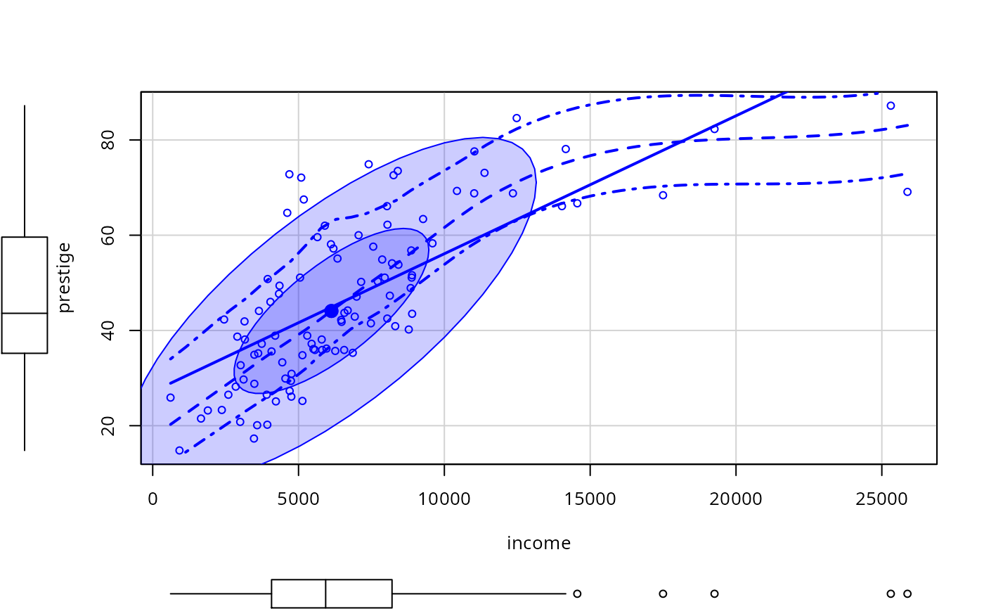
scatterplot(prestige ~ income, data=Prestige, ellipse=TRUE,
smooth=list(style="lines"))
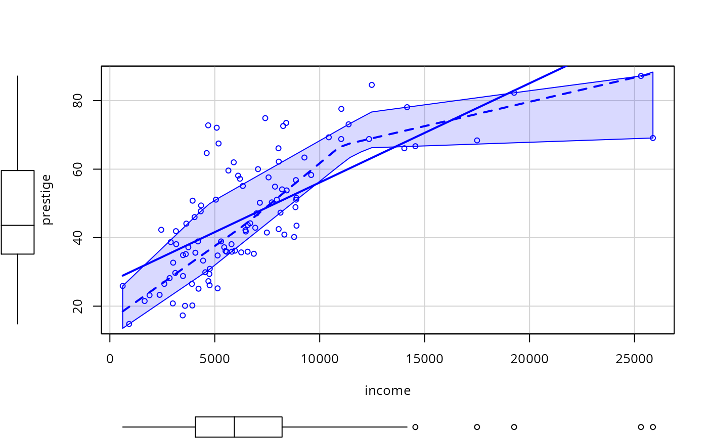
 scatterplot(prestige ~ income, data=Prestige,
smooth=list(smoother=quantregLine))
scatterplot(prestige ~ income, data=Prestige,
smooth=list(smoother=quantregLine))
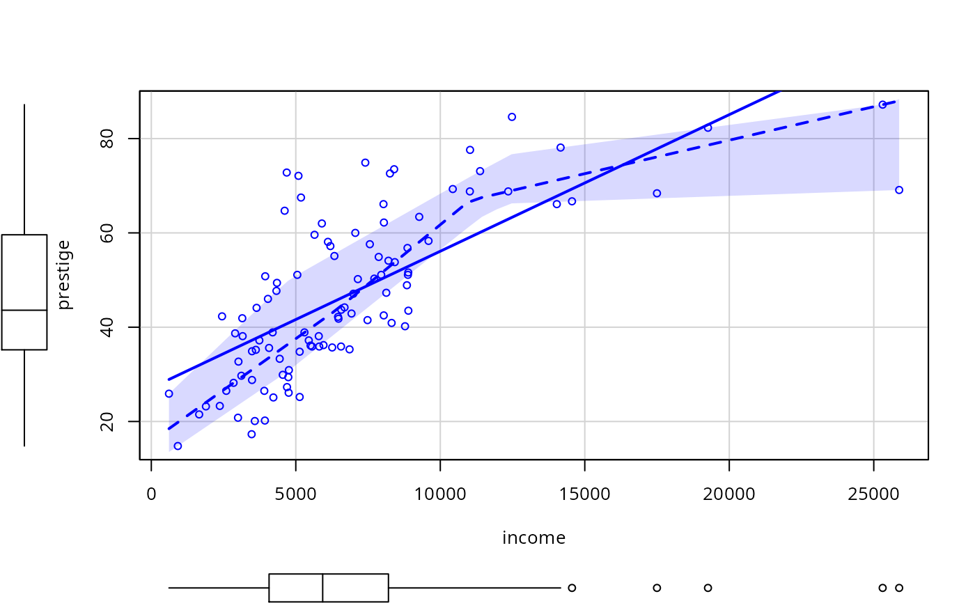
 scatterplot(prestige ~ income, data=Prestige,
smooth=list(smoother=quantregLine, border="FALSE"))
scatterplot(prestige ~ income, data=Prestige,
smooth=list(smoother=quantregLine, border="FALSE"))
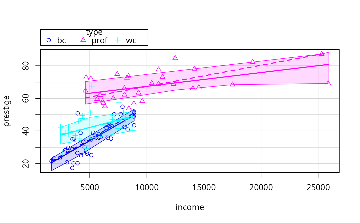
 # use quantile regression for median and quartile fits
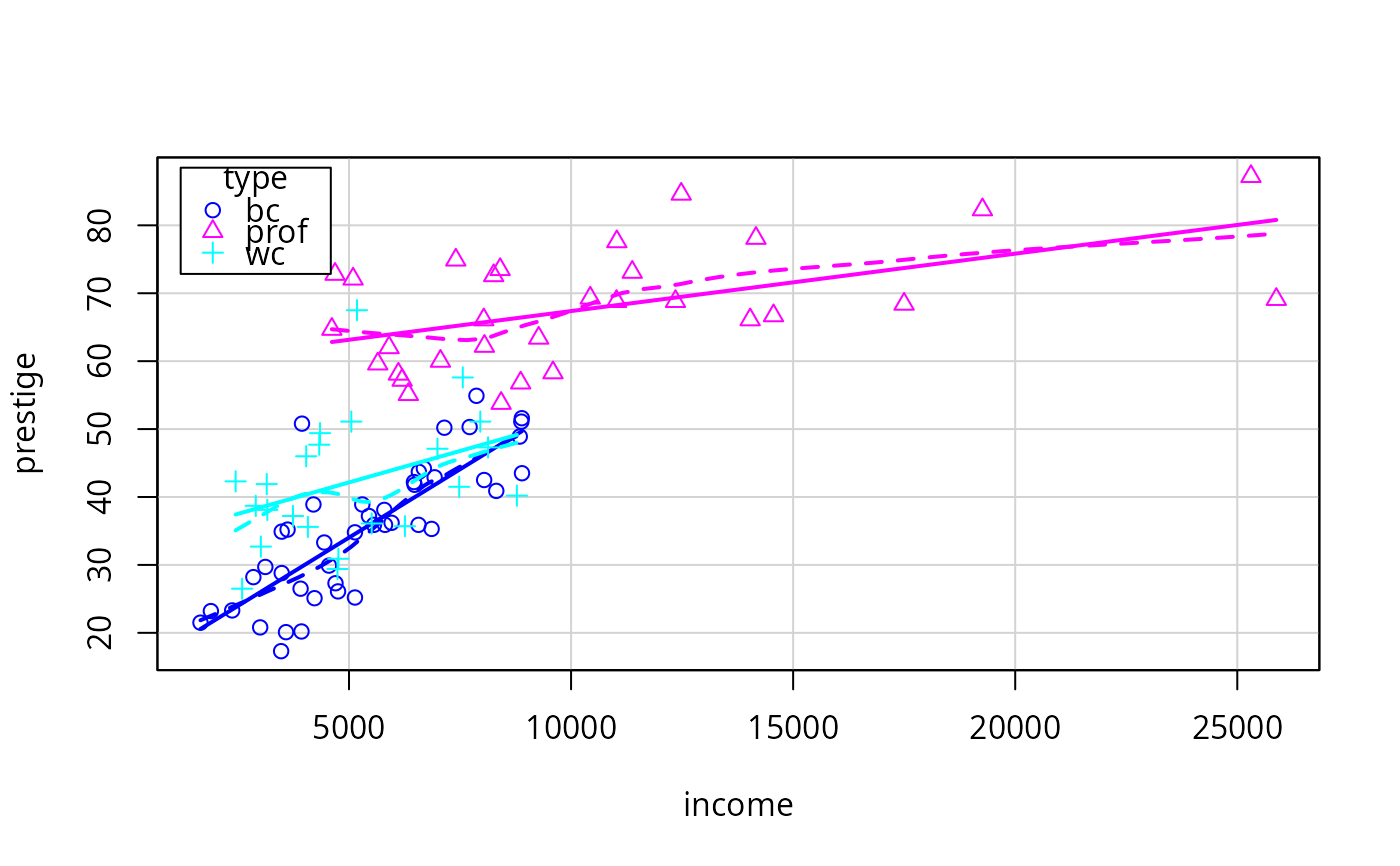
scatterplot(prestige ~ income | type, data=Prestige,
smooth=list(smoother=quantregLine, var=TRUE, span=1, lwd=4, lwd.var=2))
# use quantile regression for median and quartile fits
scatterplot(prestige ~ income | type, data=Prestige,
smooth=list(smoother=quantregLine, var=TRUE, span=1, lwd=4, lwd.var=2))
 scatterplot(prestige ~ income | type, data=Prestige,
legend=list(coords="topleft"))
scatterplot(prestige ~ income | type, data=Prestige,
legend=list(coords="topleft"))
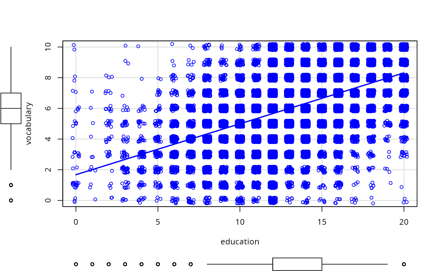
 scatterplot(vocabulary ~ education, jitter=list(x=1, y=1),
data=Vocab, smooth=FALSE, lwd=3)
scatterplot(vocabulary ~ education, jitter=list(x=1, y=1),
data=Vocab, smooth=FALSE, lwd=3)
 scatterplot(infantMortality ~ ppgdp, log="xy", data=UN, id=list(n=5))
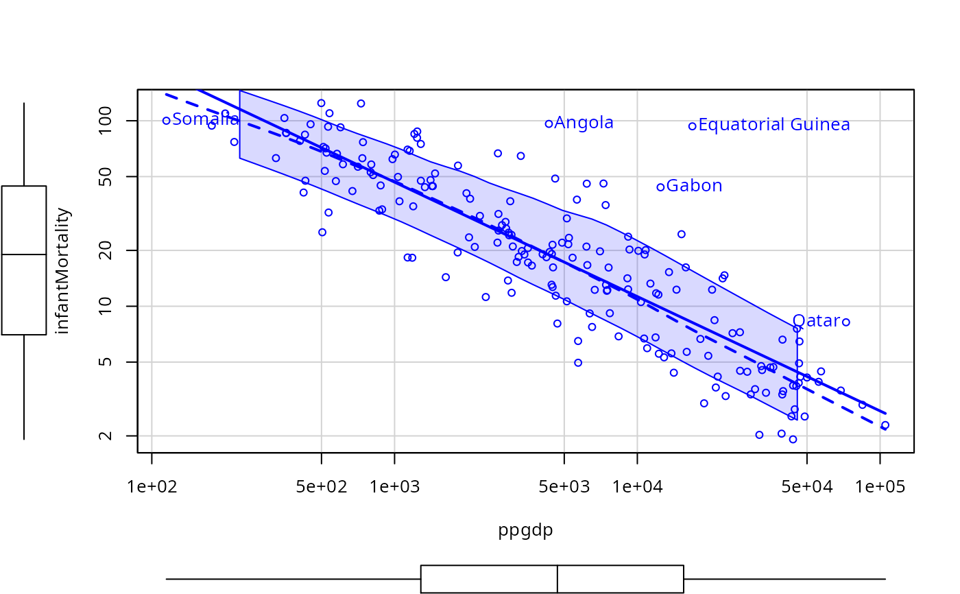 #> Angola Equatorial Guinea Gabon Qatar
#> 4 54 62 143
#> Somalia
#> 159
scatterplot(income ~ type, data=Prestige)
#> Angola Equatorial Guinea Gabon Qatar
#> 4 54 62 143
#> Somalia
#> 159
scatterplot(income ~ type, data=Prestige)
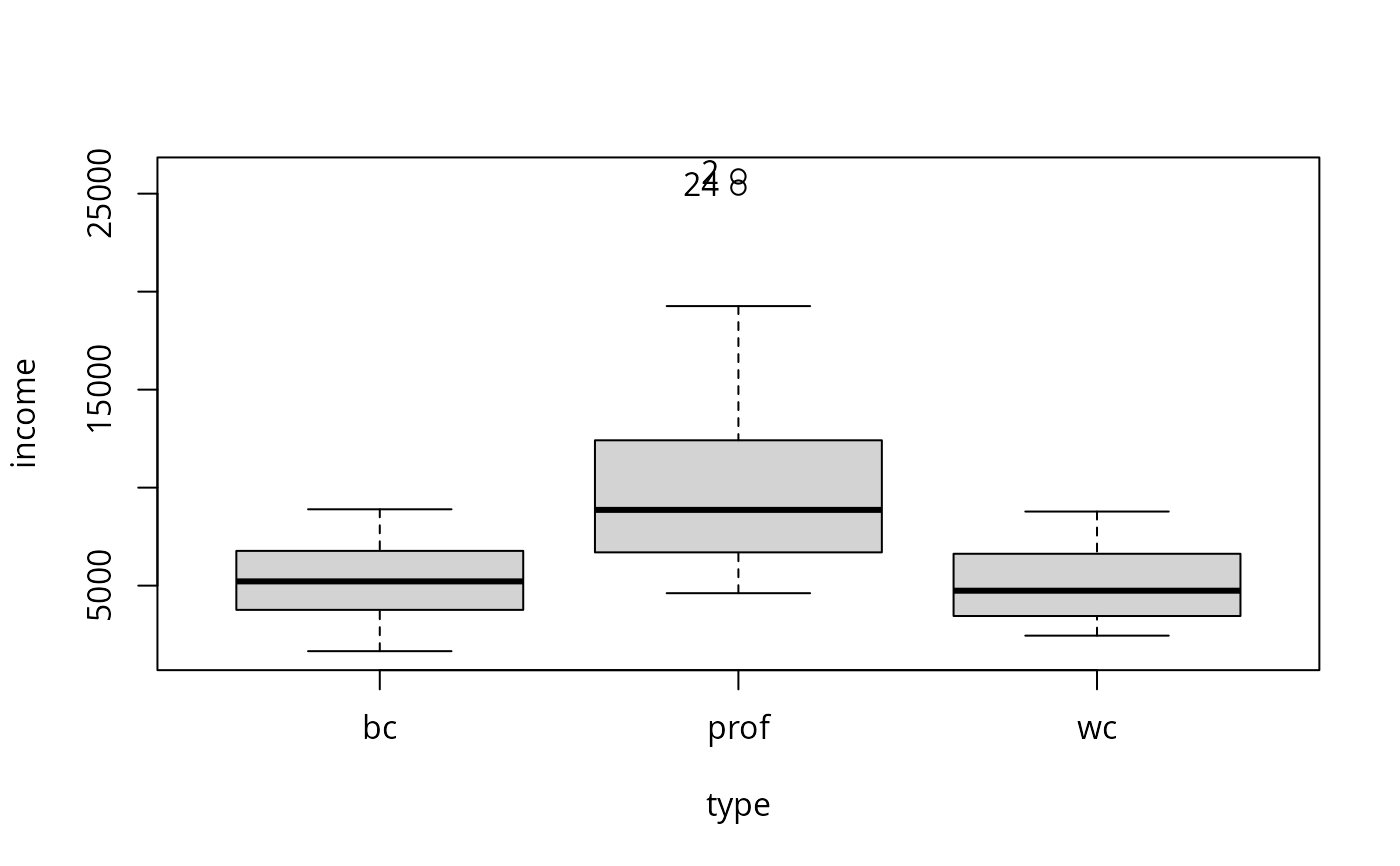 #> [1] "2" "24"
if (FALSE) # interactive point identification
# remember to exit from point-identification mode
scatterplot(infantMortality ~ ppgdp, id=list(method="identify"), data=UN)
# \dontrun{}
#> [1] "2" "24"
if (FALSE) # interactive point identification
# remember to exit from point-identification mode
scatterplot(infantMortality ~ ppgdp, id=list(method="identify"), data=UN)
# \dontrun{}