Generic function for plotting regressions and interaction effects
plotSlopes.RdThis is a function for plotting regression
objects. So far, there is an implementation for lm() objects.
I've been revising plotSlopes so that it should handle the work
performed by plotCurves. As sure as that belief is verified,
the plotCurves work will be handled by plotSlopes. Different
plot types are created, depending on whether the x-axis predictor
plotx is numeric or categorical.
##'
This is a "simple slope" plotter for regression objects created by
lm() or similar functions that have capable predict methods
with newdata arguments. The term "simple slopes" was coined by
psychologists (Aiken and West, 1991; Cohen, et al 2002) for
analysis of interaction effects for particular values of a
moderating variable. The moderating variable may be continuous or
categorical, lines will be plotted for focal values of that
variable.
Usage
plotSlopes(model, plotx, ...)

# S3 method for class 'lm'
plotSlopes(
  model,
  plotx,
  modx = NULL,
  n = 3,
  modxVals = NULL,
  plotxRange = NULL,
  interval = c("none", "confidence", "prediction"),
  plotPoints = TRUE,
  legendPct = TRUE,
  legendArgs,
  llwd = 2,
  opacity = 100,
  ...,
  col = c("black", "blue", "darkgreen", "red", "orange", "purple", "green3"),
  type = c("response", "link"),
  gridArgs,
  width = 0.2
)
Arguments
- model
Required. A fitted Regression
- plotx
Required. Name of one predictor from the fitted model to be plotted on horizontal axis. May be numeric or factor.
- ...
Additional arguments passed to methods. Often includes arguments that are passed to plot. Any arguments that customize plot output, such as lwd, cex, and so forth, may be supplied. These arguments intended for the predict method will be used: c("type", "se.fit", "interval", "level", "dispersion", "terms", "na.action")
- modx
Optional. String for moderator variable name. May be either numeric or factor. If omitted, a single predicted value line will be drawn.
- n
Optional. Number of focal values of
modx, used by algorithms specified by modxVals; will be ignored if modxVals supplies a vector of focal values.- modxVals
Optional. Focal values of
modxfor which lines are desired. May be a vector of values or the name of an algorithm, "quantile", "std.dev.", or "table".- plotxRange
Optional. If not specified, the observed range of plotx will be used to determine the axis range.
- interval
Optional. Intervals provided by the
predict.lmmay be supplied, either "confidence" (confidence interval for the estimated conditional mean) or "prediction" (interval for observed values of y given the rest of the model). The level can be specified as an argument (which goes into ... and then to the predict method)- plotPoints
Optional. TRUE or FALSE: Should the plot include the scatterplot points along with the lines.
- legendPct
Default = TRUE. Variable labels print with sample percentages.
- legendArgs
Set as "none" if no legend is desired. Otherwise, this can be a list of named arguments that will override the settings I have for the legend.
- llwd
Optional, default = 2. Line widths for predicted values. Can be single value or a vector, which will be recycled as necessary.
- opacity
Optional, default = 100. A number between 1 and 255. 1 means "transparent" or invisible, 255 means very dark. Determines the darkness of confidence interval regions
- col
Optional.I offer my preferred color vector as default. Replace if you like. User may supply a vector of valid color names, or
rainbow(10)orgray.colors(5). Color names will be recycled if there are more focal values ofmodxthan colors provided.- type
Argument passed to the predict function. If model is glm, can be either "response" or "link". For lm, no argument of this type is needed, since both types have same value.
- gridArgs
Only used if plotx (horizontal axis) is a factor variable. Designates reference lines between values. Set as "none" if no grid lines are needed. Default will be
gridArgs = list(lwd = 0.3, lty = 5)- width
Only used if plotx (horizontal axis) is a factor. Designates thickness of shading for bars that depict confidence intervals.
Value
Creates a plot and an output object that summarizes it.
The return object includes the "newdata" object that was used to create the plot, along with the "modxVals" vector, the values of the moderator for which lines were drawn, and the color vector. It also includes the call that generated the plot.
Details
The original plotSlopes did not work well with nonlinear
predictors (log(x) and poly(x)). The separate function
plotCurves() was created for nonlinear predictive equations
and generalized linear models, but the separation of the two
functions was confusing for users. I've been working to make
plotSlopes handle everything and plotCurves will disappear
at some point. plotSlopes can create an object which
is then tested with testSlopes() and that can be graphed
by a plot method.
The argument plotx is the name of the horizontal plotting
variable. An innovation was introduced in Version 1.8.33 so that
plotx can be either numeric or categorical.
The argument modx is the moderator variable. It may be
either a numeric or a factor variable. As of version 1.7, the modx
argument may be omitted. A single predicted value line will be
drawn. That version also introduced the arguments interval and n.
There are many ways to specify focal values using the arguments
modxVals and n. This changed in rockchalk-1.7.0. If
modxVals is omitted, a default algorithm for the variable
type will be used to select n values for
plotting. modxVals may be a vector of values (for a numeric
moderator) or levels (for a factor). If modxVals is a vector of
values, then the argument n is ignored. However, if
modxVals is one of the name of one of the algorithms, "table",
"quantile", or "std.dev.", then the argument n sets number
of focal values to be selected. For numeric modx, n
defaults to 3, but for factors modx will be the number of
observed values of modx. If modxVals is omitted, the
defaults will be used ("table" for factors, "quantile" for numeric
variables).
For the predictors besides modx and plotx (the ones
that are not explicitly included in the plot), predicted values
are calculated with variables set to the mean and mode, for numeric
or factor variables (respectively). Those values can be reviewed
in the newdata object that is created as a part of the output from
this function
References
Aiken, L. S. and West, S.G. (1991). Multiple Regression: Testing and Interpreting Interactions. Newbury Park, Calif: Sage Publications.
Cohen, J., Cohen, P., West, S. G., and Aiken, L. S. (2002). Applied Multiple Regression/Correlation Analysis for the Behavioral Sciences (Third.). Routledge Academic.
Author
Paul E. Johnson pauljohn@ku.edu
Examples
## Manufacture some predictors
set.seed(12345)
dat <- genCorrelatedData2 (N = 100, means = rep(0,4), sds = 1, rho = 0.2,
beta = c(0.3, 0.5, -0.45, 0.5, -0.1, 0, 0.6),
stde = 2)
#> [1] "The equation that was calculated was"
#> y = 0.3 + 0.5*x1 + -0.45*x2 + 0.5*x3 + -0.1*x4
#> + 0*x1*x1 + 0.6*x2*x1 + 0*x3*x1 + 0*x4*x1
#> + 0*x1*x2 + 0*x2*x2 + 0*x3*x2 + 0*x4*x2
#> + 0*x1*x3 + 0*x2*x3 + 0*x3*x3 + 0*x4*x3
#> + 0*x1*x4 + 0*x2*x4 + 0*x3*x4 + 0*x4*x4
#> + N(0,2) random error
dat$xcat1 <- gl(2, 50, labels = c("M", "F"))
dat$xcat2 <- cut(rnorm(100), breaks = c(-Inf, 0, 0.4, 0.9, 1, Inf),
labels = c("R", "M", "D", "P", "G"))
## incorporate effect of categorical predictors
dat$y <- dat$y + 1.9 * dat$x1 * contrasts(dat$xcat1)[dat$xcat1] +
contrasts(dat$xcat2)[dat$xcat2 , ] %*% c(0.1, -0.16, 0, 0.2)
m1 <- lm(y ~ x1 * x2 + x3 + x4 + xcat1* xcat2, data = dat)
summary(m1)
#>
#> Call:
#> lm(formula = y ~ x1 * x2 + x3 + x4 + xcat1 * xcat2, data = dat)
#>
#> Residuals:
#> Min 1Q Median 3Q Max
#> -4.875 -1.298 -0.092 1.208 4.502
#>
#> Coefficients:
#> Estimate Std. Error t value Pr(>|t|)
#> (Intercept) 0.3240 0.4188 0.774 0.441297
#> x1 0.7849 0.2135 3.675 0.000410 ***
#> x2 -0.4008 0.2141 -1.872 0.064583 .
#> x3 0.5935 0.2328 2.550 0.012524 *
#> x4 0.3370 0.2140 1.575 0.118880
#> xcat1F -0.3633 0.5924 -0.613 0.541295
#> xcat2M 0.6850 1.1027 0.621 0.536082
#> xcat2D 0.1059 0.6927 0.153 0.878831
#> xcat2G 1.1424 0.8786 1.300 0.196933
#> x1:x2 0.9011 0.2228 4.045 0.000113 ***
#> xcat1F:xcat2M 0.7264 1.4670 0.495 0.621710
#> xcat1F:xcat2D -1.0294 0.9980 -1.031 0.305172
#> xcat1F:xcat2G -0.6250 1.1961 -0.523 0.602615
#> ---
#> Signif. codes: 0 ‘***’ 0.001 ‘**’ 0.01 ‘*’ 0.05 ‘.’ 0.1 ‘ ’ 1
#>
#> Residual standard error: 2.005 on 87 degrees of freedom
#> Multiple R-squared: 0.4383, Adjusted R-squared: 0.3608
#> F-statistic: 5.657 on 12 and 87 DF, p-value: 4.311e-07
#>
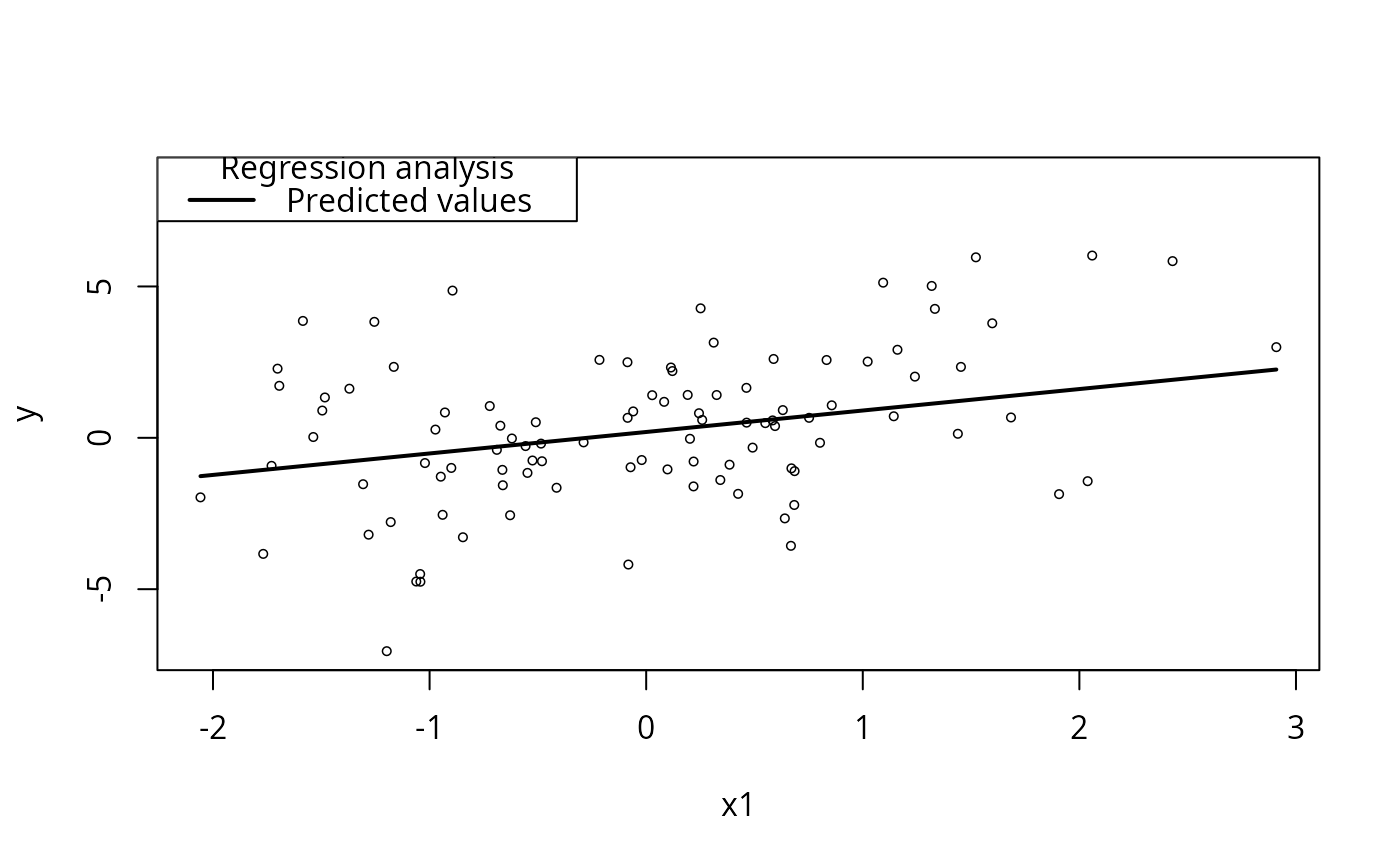
## New in rockchalk 1.7.x. No modx required:
plotSlopes(m1, plotx = "x1")
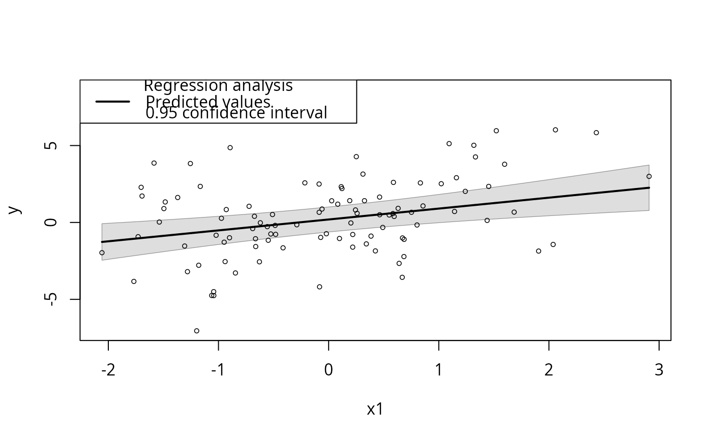
 ## Confidence interval, anybody?
plotSlopes(m1, plotx = "x1", interval = "conf")
## Confidence interval, anybody?
plotSlopes(m1, plotx = "x1", interval = "conf")
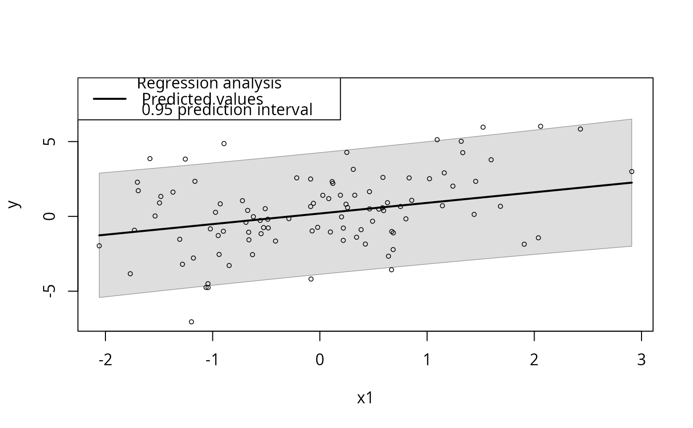
 ## Prediction interval.
plotSlopes(m1, plotx = "x1", interval = "pred")
## Prediction interval.
plotSlopes(m1, plotx = "x1", interval = "pred")
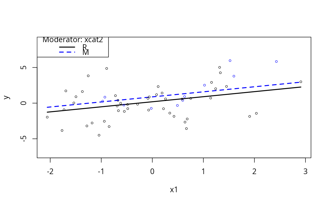
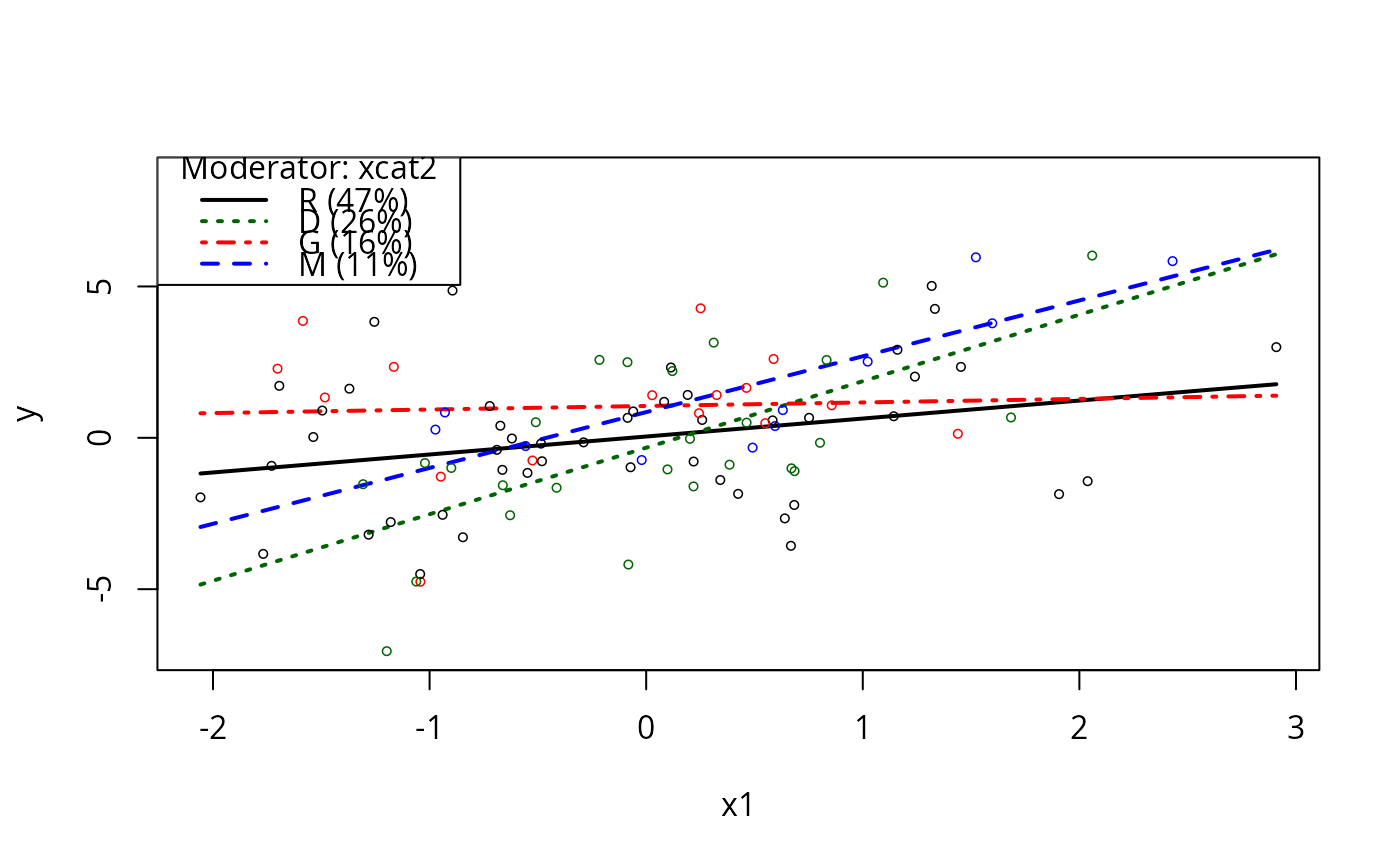
 plotSlopes(m1, plotx = "x1", modx = "xcat2", modxVals = c("R", "M"))
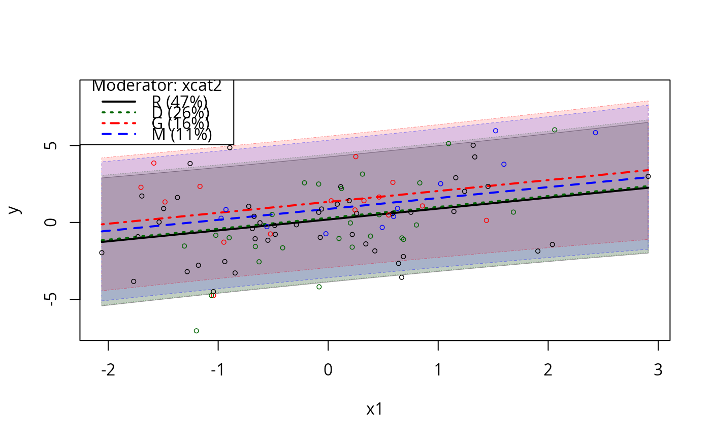
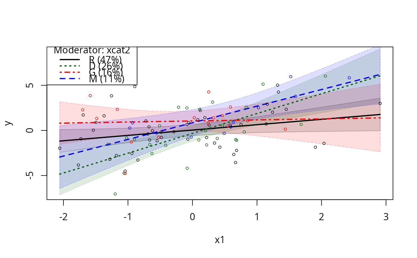
 plotSlopes(m1, plotx = "x1", modx = "xcat2", interval = "pred")
 plotSlopes(m1, plotx = "xcat1", modx = "xcat2", interval = "conf", space = c(0,1))
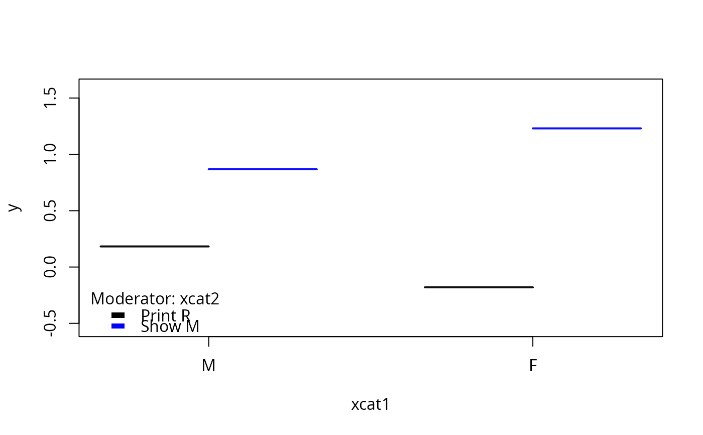
 plotSlopes(m1, plotx = "xcat1", modx = "xcat2",
modxVals = c("Print R" = "R" , "Show M" = "M"), gridArgs = "none")
plotSlopes(m1, plotx = "xcat1", modx = "xcat2",
modxVals = c("Print R" = "R" , "Show M" = "M"), gridArgs = "none")
 ## Now experiment with a moderator variable
## let default quantile algorithm do its job
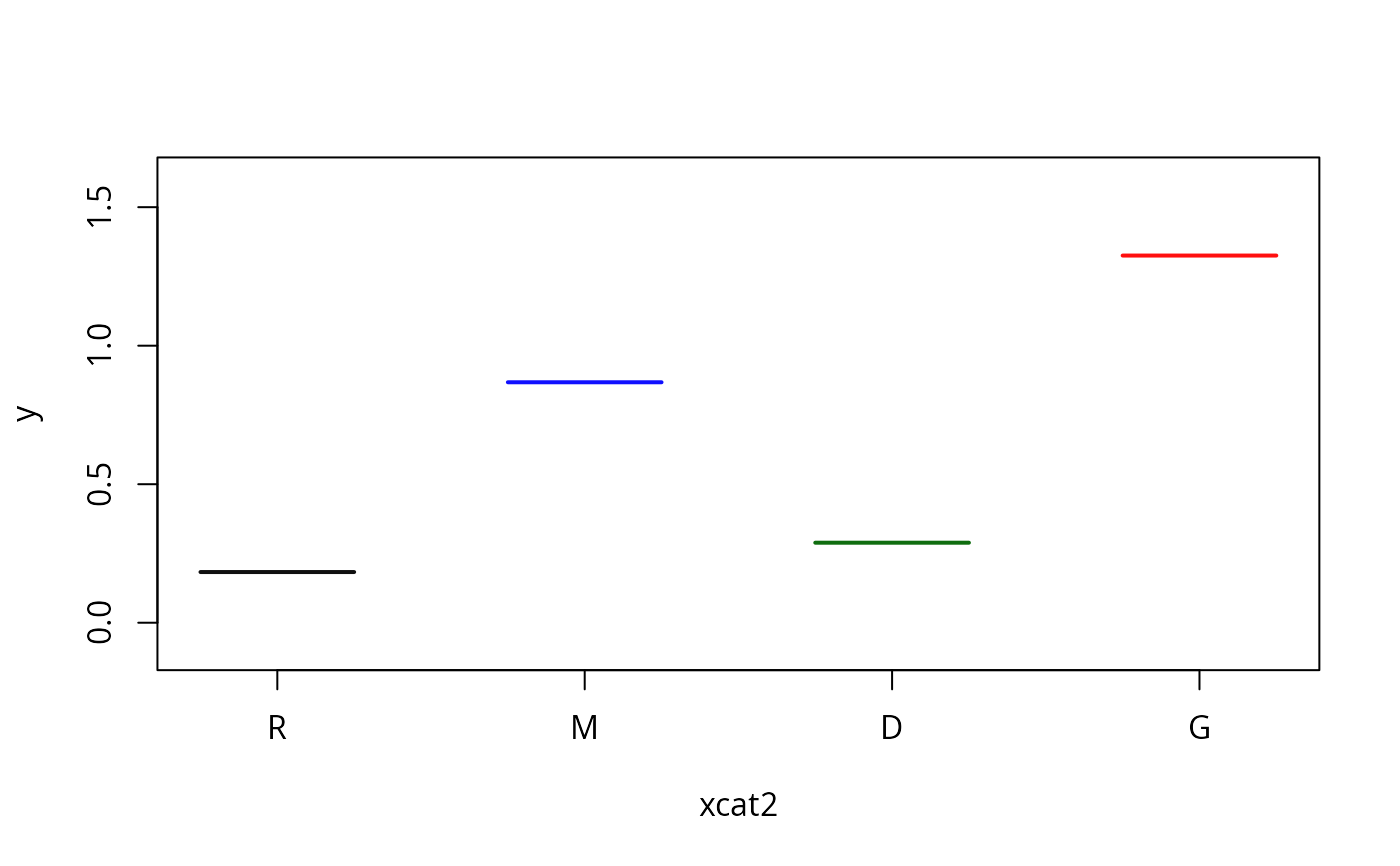
plotSlopes(m1, plotx = "xcat2", interval = "none")
## Now experiment with a moderator variable
## let default quantile algorithm do its job
plotSlopes(m1, plotx = "xcat2", interval = "none")
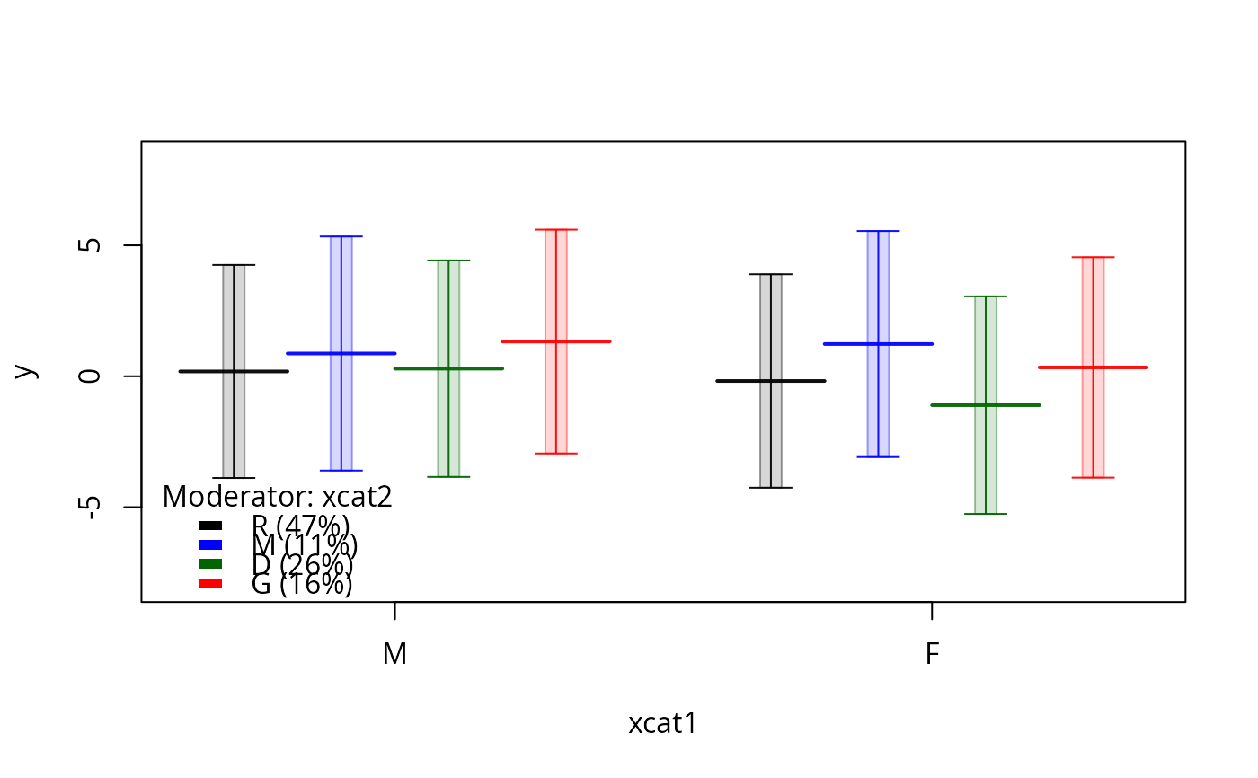
 plotSlopes(m1, plotx = "xcat1", modx = "xcat2", interval = "none")
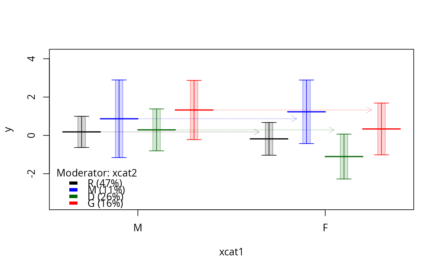
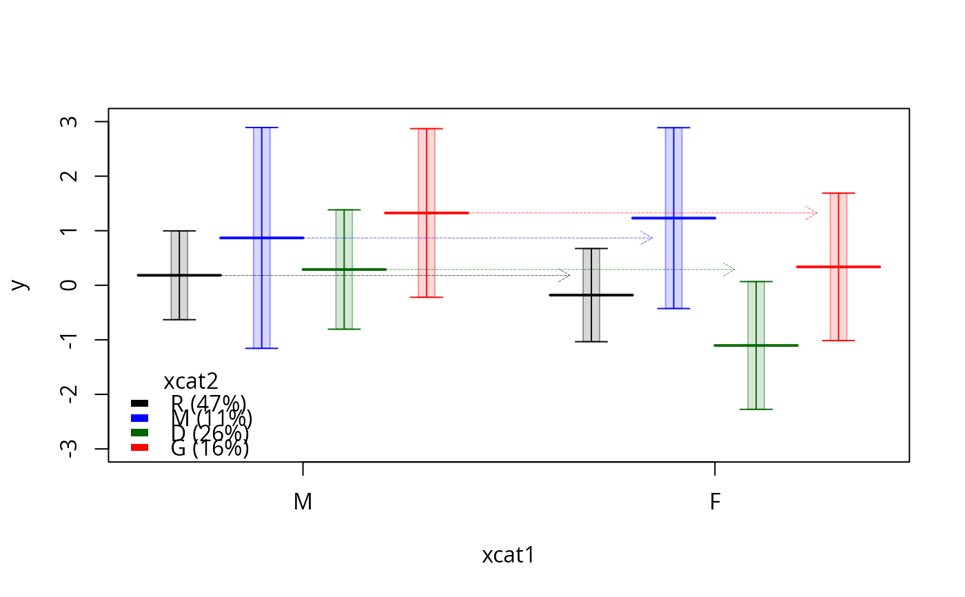
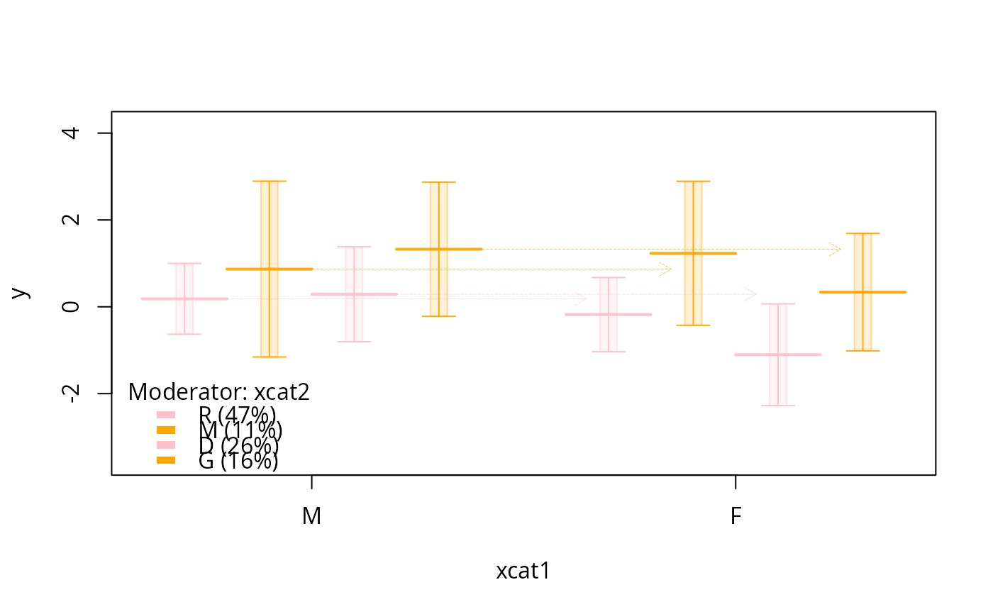
 plotSlopes(m1, plotx = "xcat1", modx = "xcat2", interval = "confidence",
legendArgs = list(title = "xcat2"), ylim = c(-3, 3), lwd = 0.4)
plotSlopes(m1, plotx = "xcat1", modx = "xcat2", interval = "confidence",
legendArgs = list(title = "xcat2"), ylim = c(-3, 3), lwd = 0.4)
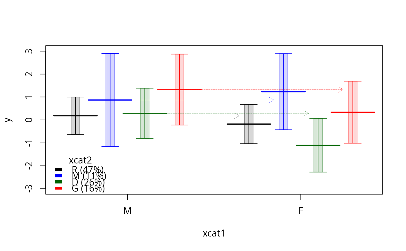
 plotSlopes(m1, plotx = "xcat1", modx = "xcat2", interval = "confidence",
legendArgs = list(title = "xcat2"), ylim = c(-3, 3), lwd = 0.4, width = 0.25)
plotSlopes(m1, plotx = "xcat1", modx = "xcat2", interval = "confidence",
legendArgs = list(title = "xcat2"), ylim = c(-3, 3), lwd = 0.4, width = 0.25)
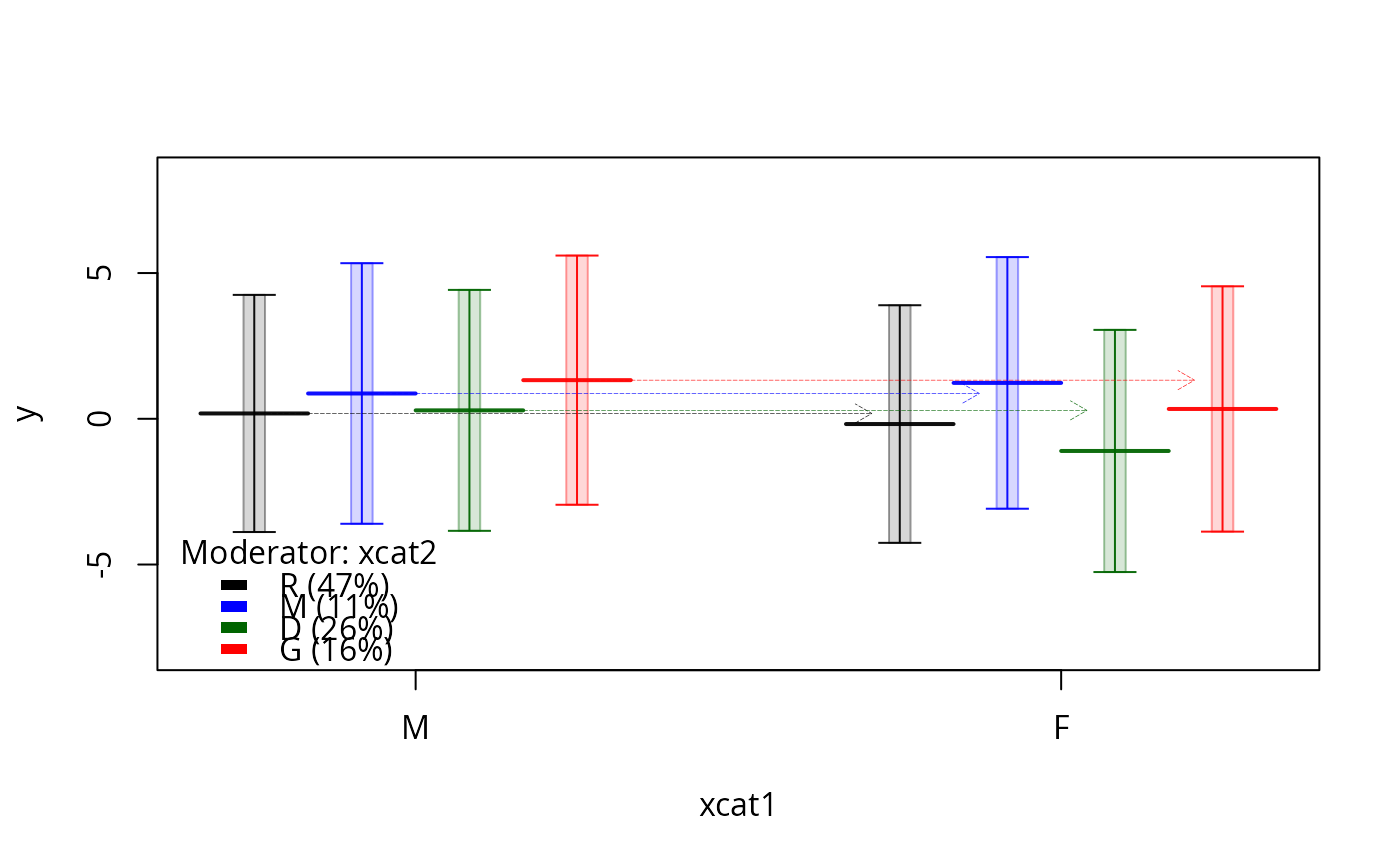
 m1.ps <- plotSlopes(m1, plotx = "xcat1", modx = "xcat2", interval = "prediction")
 m1.ps <- plotSlopes(m1, plotx = "xcat1", modx = "xcat2", interval = "prediction", space=c(0,2))
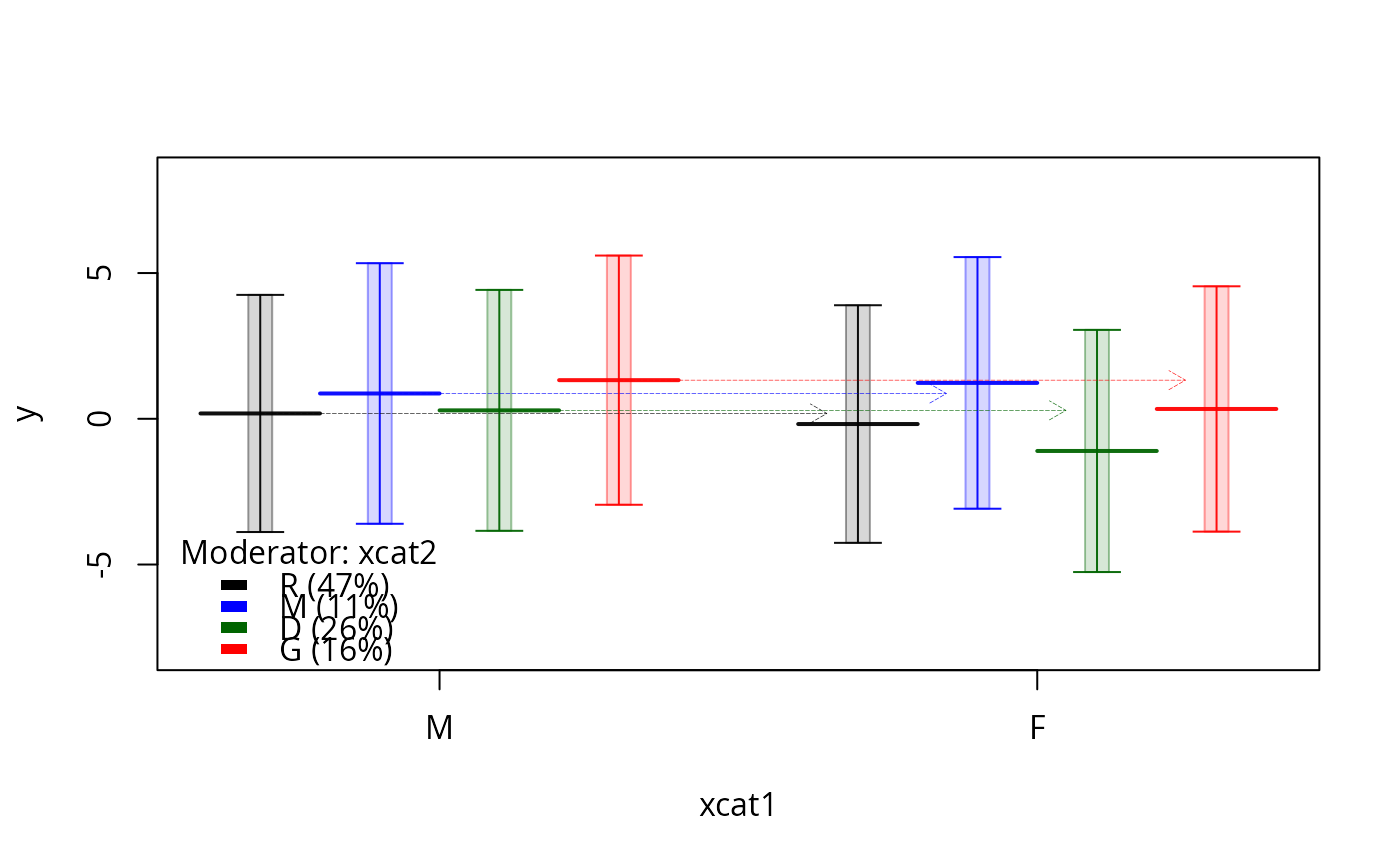
 plotSlopes(m1, plotx = "xcat1", modx = "xcat2", interval = "prediction", gridArgs = "none")
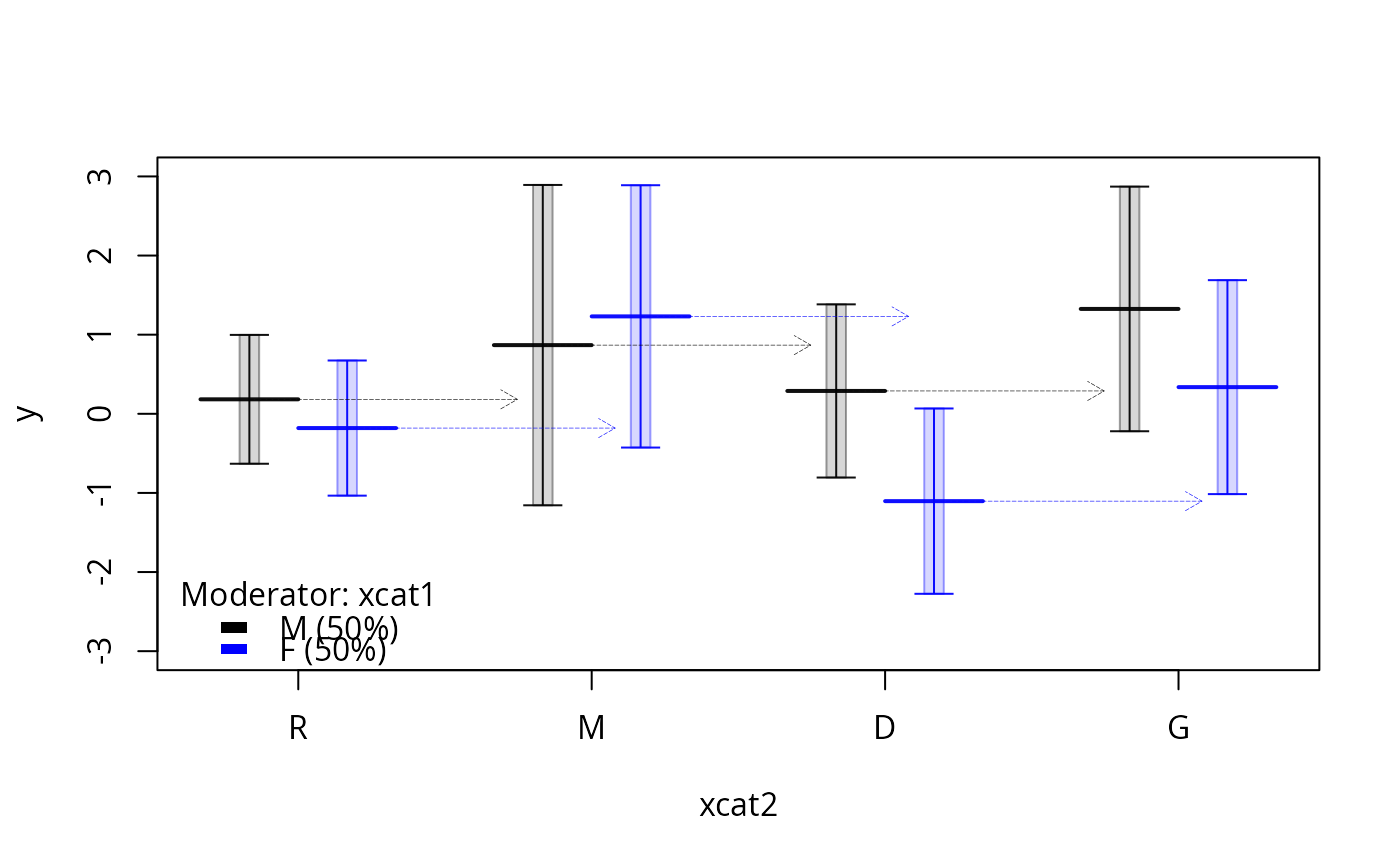
 plotSlopes(m1, plotx = "xcat2", modx = "xcat1", interval = "confidence", ylim = c(-3, 3))
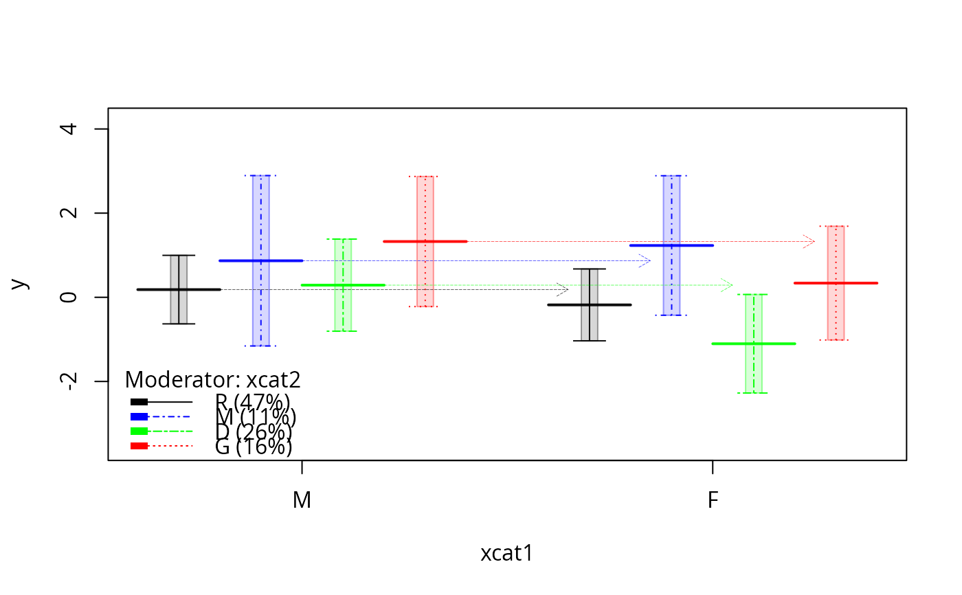
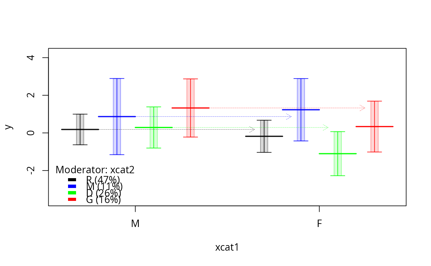
 plotSlopes(m1, plotx = "xcat1", modx = "xcat2", interval = "confidence",
col = c("black", "blue", "green", "red", "orange"), lty = c(1, 4, 6, 3))
plotSlopes(m1, plotx = "xcat1", modx = "xcat2", interval = "confidence",
col = c("black", "blue", "green", "red", "orange"), lty = c(1, 4, 6, 3))
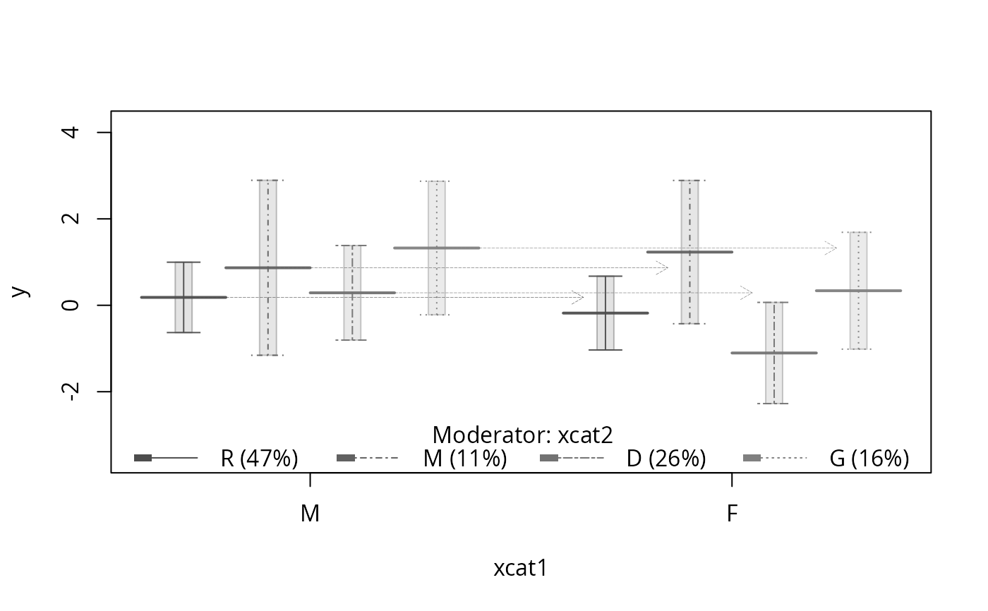
 plotSlopes(m1, plotx = "xcat1", modx = "xcat2", interval = "confidence",
col = gray.colors(4, end = 0.5), lty = c(1, 4, 6, 3), legendArgs = list(horiz=TRUE))
plotSlopes(m1, plotx = "xcat1", modx = "xcat2", interval = "confidence",
col = gray.colors(4, end = 0.5), lty = c(1, 4, 6, 3), legendArgs = list(horiz=TRUE))
 plotSlopes(m1, plotx = "xcat1", modx = "xcat2", interval = "confidence",
col = c("pink", "orange"))
plotSlopes(m1, plotx = "xcat1", modx = "xcat2", interval = "confidence",
col = c("pink", "orange"))
 plotSlopes(m1, plotx = "xcat1", interval = "confidence",
col = c("black", "blue", "green", "red", "orange"))
plotSlopes(m1, plotx = "xcat1", interval = "confidence",
col = c("black", "blue", "green", "red", "orange"))
 plotSlopes(m1, plotx = "xcat1", modx = "xcat2", interval = "confidence",
col = c("black", "blue", "green", "red", "orange"),
gridlwd = 0.2)
plotSlopes(m1, plotx = "xcat1", modx = "xcat2", interval = "confidence",
col = c("black", "blue", "green", "red", "orange"),
gridlwd = 0.2)
 ## previous uses default equivalent to
## plotSlopes(m1, plotx = "x1", modx = "x2", modxVals = "quantile")
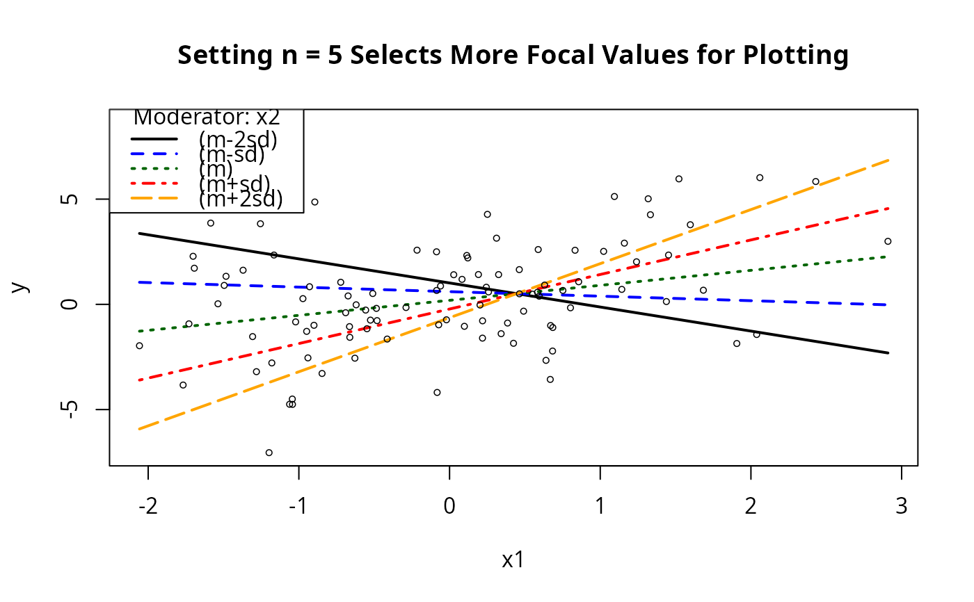
## Want more focal values?
plotSlopes(m1, plotx = "x1", modx = "x2", n = 5)
## previous uses default equivalent to
## plotSlopes(m1, plotx = "x1", modx = "x2", modxVals = "quantile")
## Want more focal values?
plotSlopes(m1, plotx = "x1", modx = "x2", n = 5)
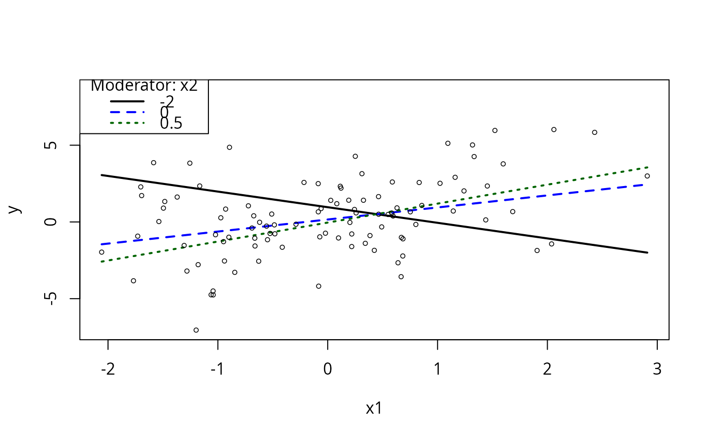
 ## Pick focal values yourself?
plotSlopes(m1, plotx = "x1", modx = "x2", modxVals = c(-2, 0, 0.5))
## Pick focal values yourself?
plotSlopes(m1, plotx = "x1", modx = "x2", modxVals = c(-2, 0, 0.5))
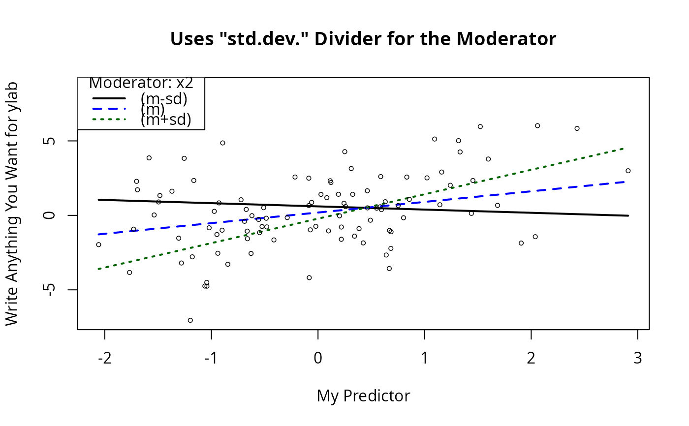
 ## Alternative algorithm?
plotSlopes(m1, plotx = "x1", modx = "x2", modxVals = "std.dev.",
main = "Uses \"std.dev.\" Divider for the Moderator",
xlab = "My Predictor", ylab = "Write Anything You Want for ylab")
## Alternative algorithm?
plotSlopes(m1, plotx = "x1", modx = "x2", modxVals = "std.dev.",
main = "Uses \"std.dev.\" Divider for the Moderator",
xlab = "My Predictor", ylab = "Write Anything You Want for ylab")
 ## Will catch output object from this one
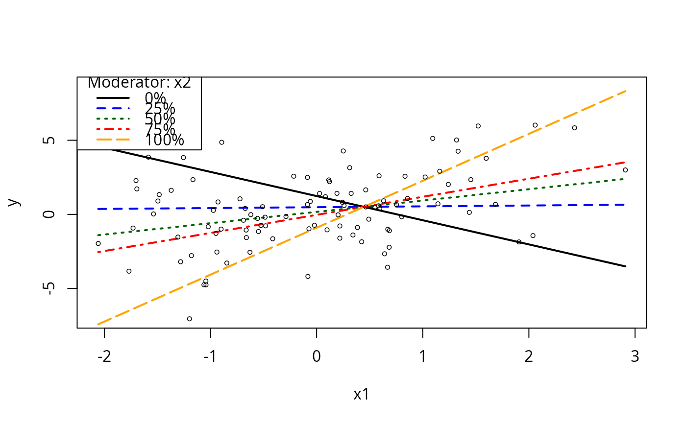
m1ps <- plotSlopes(m1, plotx = "x1", modx = "x2", modxVals = "std.dev.", n = 5,
main = "Setting n = 5 Selects More Focal Values for Plotting")
## Will catch output object from this one
m1ps <- plotSlopes(m1, plotx = "x1", modx = "x2", modxVals = "std.dev.", n = 5,
main = "Setting n = 5 Selects More Focal Values for Plotting")
 m1ts <- testSlopes(m1ps)
#> Error in eval(parse(text = object$call$model)): object 'm1' not found
plot(m1ts)
#> Error: object 'm1ts' not found
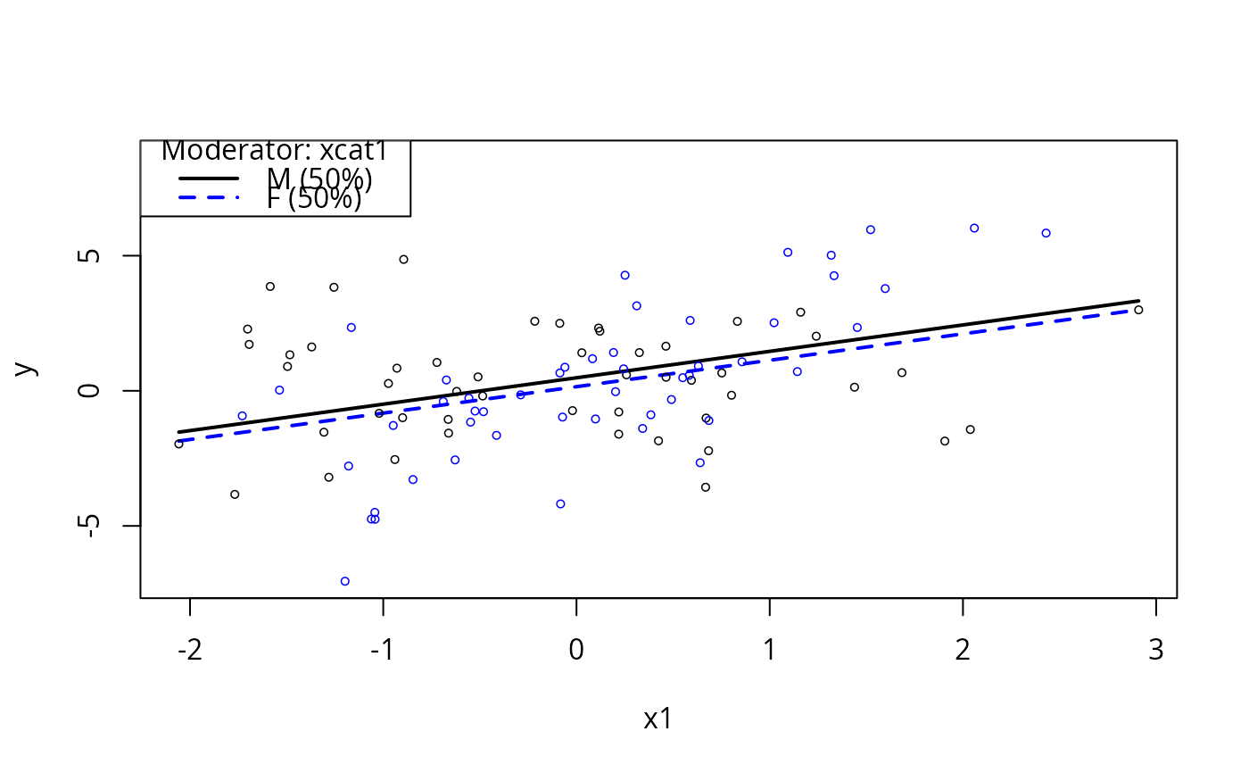
### Examples with categorical Moderator variable
m3 <- lm (y ~ x1 + xcat1, data = dat)
summary(m3)
#>
#> Call:
#> lm(formula = y ~ x1 + xcat1, data = dat)
#>
#> Residuals:
#> Min 1Q Median 3Q Max
#> -6.0286 -1.4198 -0.1459 1.3108 5.2555
#>
#> Coefficients:
#> Estimate Std. Error t value Pr(>|t|)
#> (Intercept) 0.4823 0.3289 1.466 0.146
#> x1 0.9777 0.2240 4.364 3.19e-05 ***
#> xcat1F -0.3302 0.4663 -0.708 0.481
#> ---
#> Signif. codes: 0 ‘***’ 0.001 ‘**’ 0.01 ‘*’ 0.05 ‘.’ 0.1 ‘ ’ 1
#>
#> Residual standard error: 2.316 on 97 degrees of freedom
#> Multiple R-squared: 0.1644, Adjusted R-squared: 0.1472
#> F-statistic: 9.544 on 2 and 97 DF, p-value: 0.0001645
#>
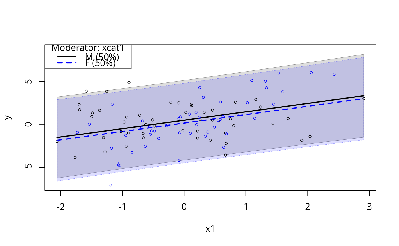
plotSlopes(m3, modx = "xcat1", plotx = "x1")
m1ts <- testSlopes(m1ps)
#> Error in eval(parse(text = object$call$model)): object 'm1' not found
plot(m1ts)
#> Error: object 'm1ts' not found
### Examples with categorical Moderator variable
m3 <- lm (y ~ x1 + xcat1, data = dat)
summary(m3)
#>
#> Call:
#> lm(formula = y ~ x1 + xcat1, data = dat)
#>
#> Residuals:
#> Min 1Q Median 3Q Max
#> -6.0286 -1.4198 -0.1459 1.3108 5.2555
#>
#> Coefficients:
#> Estimate Std. Error t value Pr(>|t|)
#> (Intercept) 0.4823 0.3289 1.466 0.146
#> x1 0.9777 0.2240 4.364 3.19e-05 ***
#> xcat1F -0.3302 0.4663 -0.708 0.481
#> ---
#> Signif. codes: 0 ‘***’ 0.001 ‘**’ 0.01 ‘*’ 0.05 ‘.’ 0.1 ‘ ’ 1
#>
#> Residual standard error: 2.316 on 97 degrees of freedom
#> Multiple R-squared: 0.1644, Adjusted R-squared: 0.1472
#> F-statistic: 9.544 on 2 and 97 DF, p-value: 0.0001645
#>
plotSlopes(m3, modx = "xcat1", plotx = "x1")
 plotSlopes(m3, modx = "xcat1", plotx = "x1", interval = "predict")
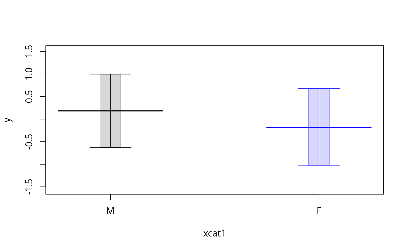
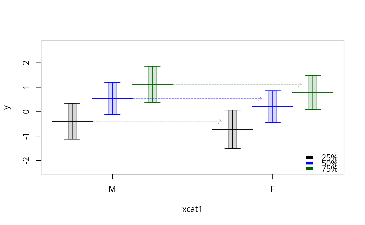
 plotSlopes(m3, modx = "x1", plotx = "xcat1", interval = "confidence",
legendArgs = list(x = "bottomright", title = ""))
plotSlopes(m3, modx = "x1", plotx = "xcat1", interval = "confidence",
legendArgs = list(x = "bottomright", title = ""))
 m4 <- lm (y ~ x1 * xcat1, data = dat)
summary(m4)
#>
#> Call:
#> lm(formula = y ~ x1 * xcat1, data = dat)
#>
#> Residuals:
#> Min 1Q Median 3Q Max
#> -4.3482 -1.3830 0.1628 1.2571 4.9690
#>
#> Coefficients:
#> Estimate Std. Error t value Pr(>|t|)
#> (Intercept) 0.35973 0.28811 1.249 0.215
#> x1 0.05296 0.25640 0.207 0.837
#> xcat1F -0.34313 0.40727 -0.843 0.402
#> x1:xcat1F 2.21447 0.39678 5.581 2.21e-07 ***
#> ---
#> Signif. codes: 0 ‘***’ 0.001 ‘**’ 0.01 ‘*’ 0.05 ‘.’ 0.1 ‘ ’ 1
#>
#> Residual standard error: 2.023 on 96 degrees of freedom
#> Multiple R-squared: 0.3691, Adjusted R-squared: 0.3494
#> F-statistic: 18.72 on 3 and 96 DF, p-value: 1.215e-09
#>
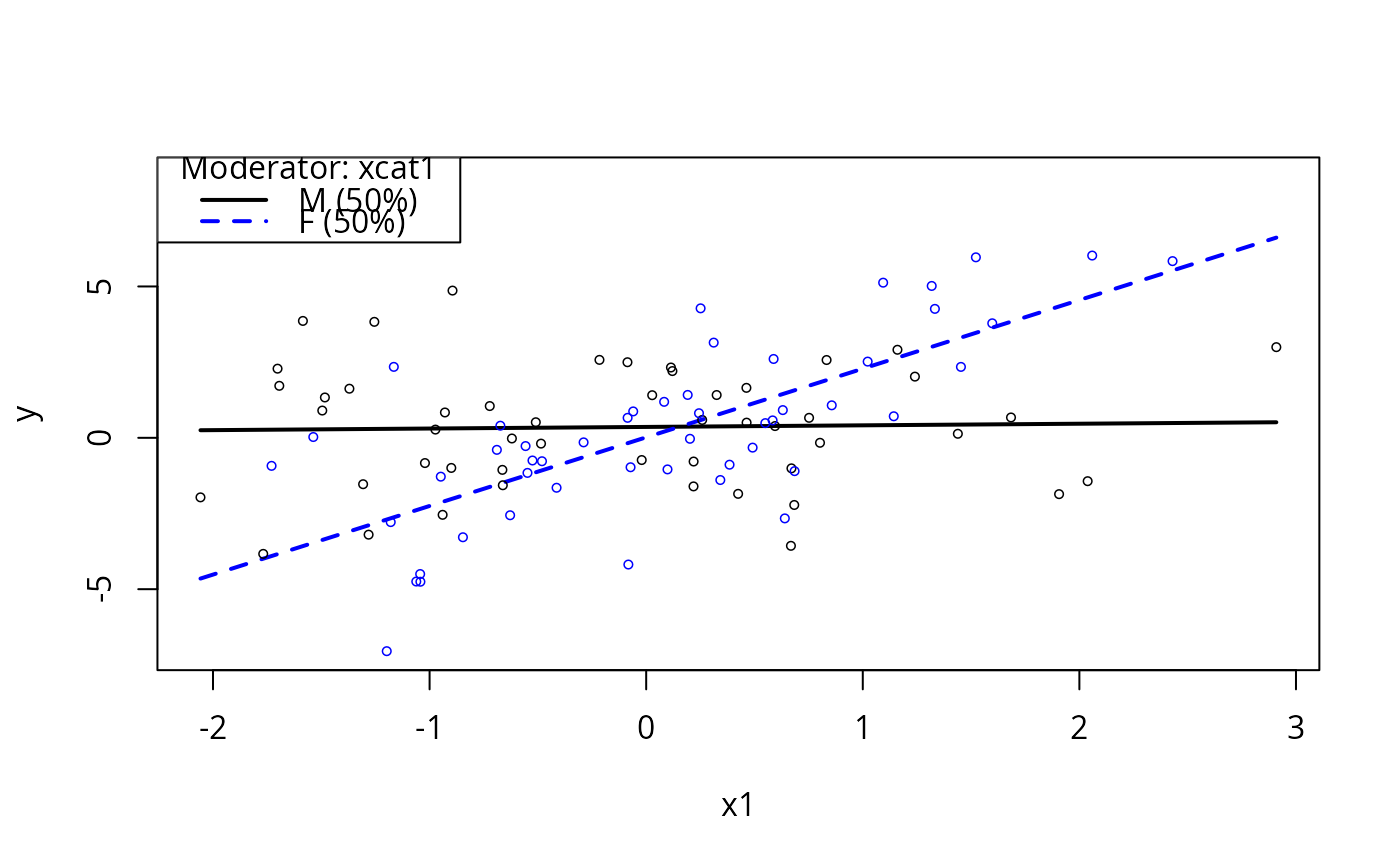
plotSlopes(m4, modx = "xcat1", plotx = "x1")
m4 <- lm (y ~ x1 * xcat1, data = dat)
summary(m4)
#>
#> Call:
#> lm(formula = y ~ x1 * xcat1, data = dat)
#>
#> Residuals:
#> Min 1Q Median 3Q Max
#> -4.3482 -1.3830 0.1628 1.2571 4.9690
#>
#> Coefficients:
#> Estimate Std. Error t value Pr(>|t|)
#> (Intercept) 0.35973 0.28811 1.249 0.215
#> x1 0.05296 0.25640 0.207 0.837
#> xcat1F -0.34313 0.40727 -0.843 0.402
#> x1:xcat1F 2.21447 0.39678 5.581 2.21e-07 ***
#> ---
#> Signif. codes: 0 ‘***’ 0.001 ‘**’ 0.01 ‘*’ 0.05 ‘.’ 0.1 ‘ ’ 1
#>
#> Residual standard error: 2.023 on 96 degrees of freedom
#> Multiple R-squared: 0.3691, Adjusted R-squared: 0.3494
#> F-statistic: 18.72 on 3 and 96 DF, p-value: 1.215e-09
#>
plotSlopes(m4, modx = "xcat1", plotx = "x1")
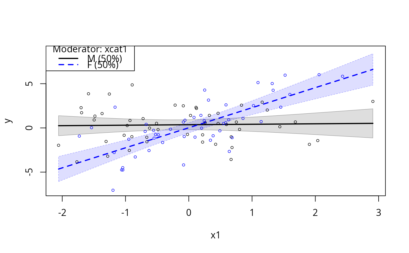
 plotSlopes(m4, modx = "xcat1", plotx = "x1", interval = "conf")
 m5 <- lm (y ~ x1 + x2 + x1 * xcat2, data = dat)
summary(m5)
#>
#> Call:
#> lm(formula = y ~ x1 + x2 + x1 * xcat2, data = dat)
#>
#> Residuals:
#> Min 1Q Median 3Q Max
#> -5.4325 -1.6743 0.0109 1.4559 5.1724
#>
#> Coefficients:
#> Estimate Std. Error t value Pr(>|t|)
#> (Intercept) 0.03088 0.31961 0.097 0.92325
#> x1 0.59372 0.28340 2.095 0.03895 *
#> x2 -0.14409 0.21884 -0.658 0.51192
#> xcat2M 0.80581 0.80778 0.998 0.32113
#> xcat2D -0.36997 0.53284 -0.694 0.48924
#> xcat2G 1.00882 0.64406 1.566 0.12074
#> x1:xcat2M 1.25047 0.69145 1.808 0.07383 .
#> x1:xcat2D 1.60326 0.57973 2.766 0.00688 **
#> x1:xcat2G -0.47664 0.64135 -0.743 0.45929
#> ---
#> Signif. codes: 0 ‘***’ 0.001 ‘**’ 0.01 ‘*’ 0.05 ‘.’ 0.1 ‘ ’ 1
#>
#> Residual standard error: 2.173 on 91 degrees of freedom
#> Multiple R-squared: 0.3103, Adjusted R-squared: 0.2496
#> F-statistic: 5.117 on 8 and 91 DF, p-value: 2.822e-05
#>
plotSlopes(m5, modx = "xcat2", plotx = "x1")
m5 <- lm (y ~ x1 + x2 + x1 * xcat2, data = dat)
summary(m5)
#>
#> Call:
#> lm(formula = y ~ x1 + x2 + x1 * xcat2, data = dat)
#>
#> Residuals:
#> Min 1Q Median 3Q Max
#> -5.4325 -1.6743 0.0109 1.4559 5.1724
#>
#> Coefficients:
#> Estimate Std. Error t value Pr(>|t|)
#> (Intercept) 0.03088 0.31961 0.097 0.92325
#> x1 0.59372 0.28340 2.095 0.03895 *
#> x2 -0.14409 0.21884 -0.658 0.51192
#> xcat2M 0.80581 0.80778 0.998 0.32113
#> xcat2D -0.36997 0.53284 -0.694 0.48924
#> xcat2G 1.00882 0.64406 1.566 0.12074
#> x1:xcat2M 1.25047 0.69145 1.808 0.07383 .
#> x1:xcat2D 1.60326 0.57973 2.766 0.00688 **
#> x1:xcat2G -0.47664 0.64135 -0.743 0.45929
#> ---
#> Signif. codes: 0 ‘***’ 0.001 ‘**’ 0.01 ‘*’ 0.05 ‘.’ 0.1 ‘ ’ 1
#>
#> Residual standard error: 2.173 on 91 degrees of freedom
#> Multiple R-squared: 0.3103, Adjusted R-squared: 0.2496
#> F-statistic: 5.117 on 8 and 91 DF, p-value: 2.822e-05
#>
plotSlopes(m5, modx = "xcat2", plotx = "x1")
 m5ps <- plotSlopes(m5, modx = "xcat2", plotx = "x1", interval = "conf")
 testSlopes(m5ps)
#> Error in eval(parse(text = object$call$model)): object 'm5' not found
## Now examples with real data. How about Chilean voters?
library(carData)
m6 <- lm(statusquo ~ income * sex, data = Chile)
summary(m6)
#>
#> Call:
#> lm(formula = statusquo ~ income * sex, data = Chile)
#>
#> Residuals:
#> Min 1Q Median 3Q Max
#> -1.78541 -0.98694 -0.04668 0.95032 1.83196
#>
#> Coefficients:
#> Estimate Std. Error t value Pr(>|t|)
#> (Intercept) 4.832e-02 3.524e-02 1.371 0.170487
#> income 3.185e-07 6.910e-07 0.461 0.644869
#> sexM -1.948e-01 5.177e-02 -3.762 0.000172 ***
#> income:sexM 1.550e-06 9.933e-07 1.561 0.118752
#> ---
#> Signif. codes: 0 ‘***’ 0.001 ‘**’ 0.01 ‘*’ 0.05 ‘.’ 0.1 ‘ ’ 1
#>
#> Residual standard error: 0.998 on 2587 degrees of freedom
#> (109 observations deleted due to missingness)
#> Multiple R-squared: 0.007461, Adjusted R-squared: 0.00631
#> F-statistic: 6.482 on 3 and 2587 DF, p-value: 0.0002283
#>
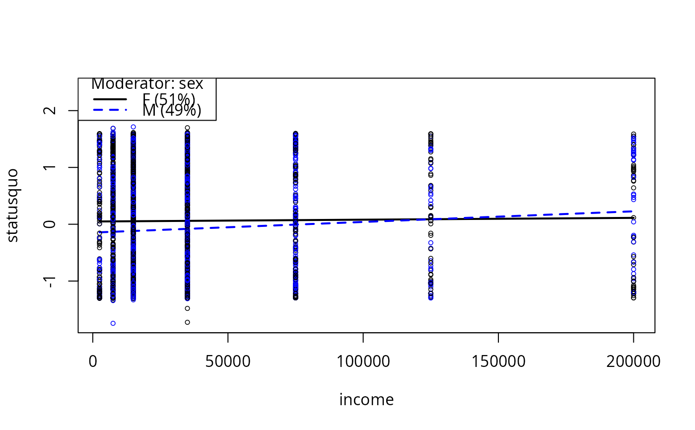
plotSlopes(m6, modx = "sex", plotx = "income")
testSlopes(m5ps)
#> Error in eval(parse(text = object$call$model)): object 'm5' not found
## Now examples with real data. How about Chilean voters?
library(carData)
m6 <- lm(statusquo ~ income * sex, data = Chile)
summary(m6)
#>
#> Call:
#> lm(formula = statusquo ~ income * sex, data = Chile)
#>
#> Residuals:
#> Min 1Q Median 3Q Max
#> -1.78541 -0.98694 -0.04668 0.95032 1.83196
#>
#> Coefficients:
#> Estimate Std. Error t value Pr(>|t|)
#> (Intercept) 4.832e-02 3.524e-02 1.371 0.170487
#> income 3.185e-07 6.910e-07 0.461 0.644869
#> sexM -1.948e-01 5.177e-02 -3.762 0.000172 ***
#> income:sexM 1.550e-06 9.933e-07 1.561 0.118752
#> ---
#> Signif. codes: 0 ‘***’ 0.001 ‘**’ 0.01 ‘*’ 0.05 ‘.’ 0.1 ‘ ’ 1
#>
#> Residual standard error: 0.998 on 2587 degrees of freedom
#> (109 observations deleted due to missingness)
#> Multiple R-squared: 0.007461, Adjusted R-squared: 0.00631
#> F-statistic: 6.482 on 3 and 2587 DF, p-value: 0.0002283
#>
plotSlopes(m6, modx = "sex", plotx = "income")
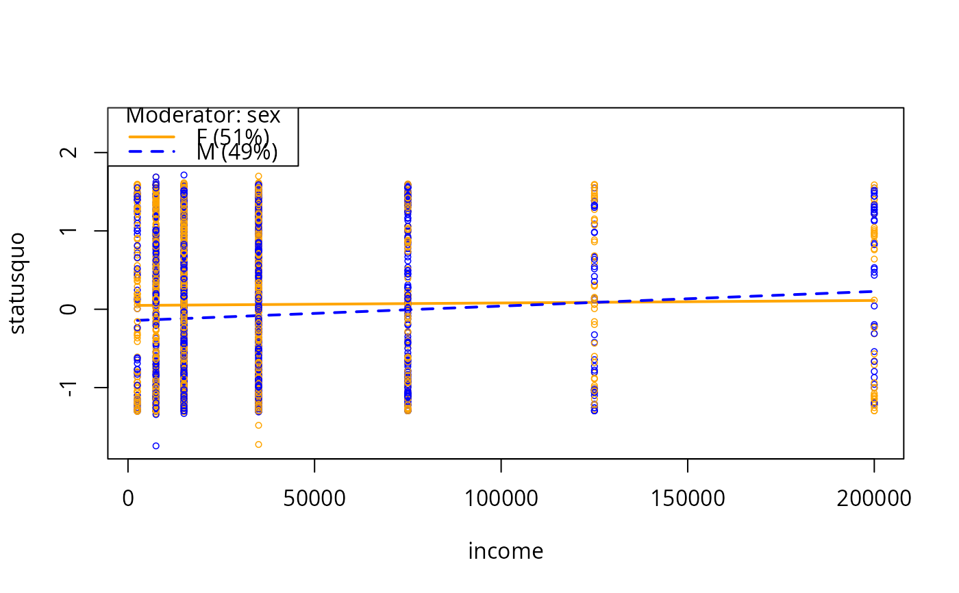
 m6ps <- plotSlopes(m6, modx = "sex", plotx = "income", col = c("orange", "blue"))
 testSlopes(m6ps)
#> Error in eval(parse(text = object$call$model)): object 'm6' not found
m7 <- lm(statusquo ~ region * income, data= Chile)
summary(m7)
#>
#> Call:
#> lm(formula = statusquo ~ region * income, data = Chile)
#>
#> Residuals:
#> Min 1Q Median 3Q Max
#> -1.87136 -0.95509 -0.05125 0.92121 1.87500
#>
#> Coefficients:
#> Estimate Std. Error t value Pr(>|t|)
#> (Intercept) -4.391e-02 5.387e-02 -0.815 0.415060
#> regionM 9.670e-02 1.613e-01 0.599 0.548985
#> regionN 8.641e-02 9.684e-02 0.892 0.372332
#> regionS 2.018e-01 7.242e-02 2.786 0.005375 **
#> regionSA -2.616e-01 6.927e-02 -3.776 0.000163 ***
#> income -4.164e-08 1.116e-06 -0.037 0.970248
#> regionM:income 9.983e-06 4.396e-06 2.271 0.023250 *
#> regionN:income 3.183e-06 2.197e-06 1.449 0.147491
#> regionS:income 3.686e-07 1.592e-06 0.232 0.816935
#> regionSA:income 2.464e-06 1.308e-06 1.884 0.059744 .
#> ---
#> Signif. codes: 0 ‘***’ 0.001 ‘**’ 0.01 ‘*’ 0.05 ‘.’ 0.1 ‘ ’ 1
#>
#> Residual standard error: 0.9847 on 2581 degrees of freedom
#> (109 observations deleted due to missingness)
#> Multiple R-squared: 0.03598, Adjusted R-squared: 0.03262
#> F-statistic: 10.7 on 9 and 2581 DF, p-value: < 2.2e-16
#>
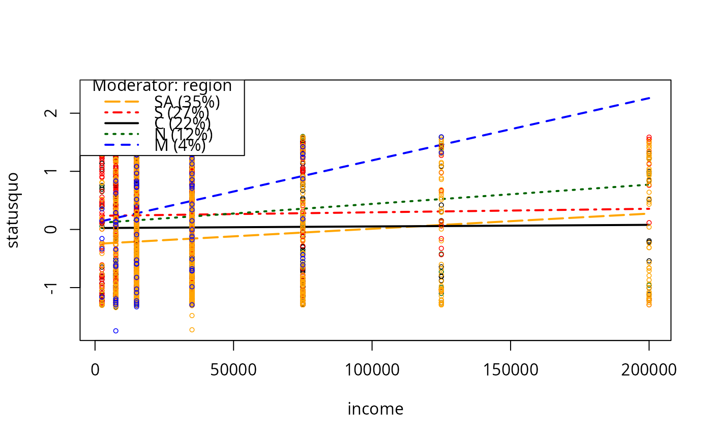
plotSlopes(m7, plotx = "income", modx = "region")
testSlopes(m6ps)
#> Error in eval(parse(text = object$call$model)): object 'm6' not found
m7 <- lm(statusquo ~ region * income, data= Chile)
summary(m7)
#>
#> Call:
#> lm(formula = statusquo ~ region * income, data = Chile)
#>
#> Residuals:
#> Min 1Q Median 3Q Max
#> -1.87136 -0.95509 -0.05125 0.92121 1.87500
#>
#> Coefficients:
#> Estimate Std. Error t value Pr(>|t|)
#> (Intercept) -4.391e-02 5.387e-02 -0.815 0.415060
#> regionM 9.670e-02 1.613e-01 0.599 0.548985
#> regionN 8.641e-02 9.684e-02 0.892 0.372332
#> regionS 2.018e-01 7.242e-02 2.786 0.005375 **
#> regionSA -2.616e-01 6.927e-02 -3.776 0.000163 ***
#> income -4.164e-08 1.116e-06 -0.037 0.970248
#> regionM:income 9.983e-06 4.396e-06 2.271 0.023250 *
#> regionN:income 3.183e-06 2.197e-06 1.449 0.147491
#> regionS:income 3.686e-07 1.592e-06 0.232 0.816935
#> regionSA:income 2.464e-06 1.308e-06 1.884 0.059744 .
#> ---
#> Signif. codes: 0 ‘***’ 0.001 ‘**’ 0.01 ‘*’ 0.05 ‘.’ 0.1 ‘ ’ 1
#>
#> Residual standard error: 0.9847 on 2581 degrees of freedom
#> (109 observations deleted due to missingness)
#> Multiple R-squared: 0.03598, Adjusted R-squared: 0.03262
#> F-statistic: 10.7 on 9 and 2581 DF, p-value: < 2.2e-16
#>
plotSlopes(m7, plotx = "income", modx = "region")
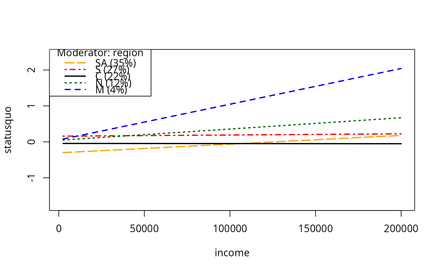
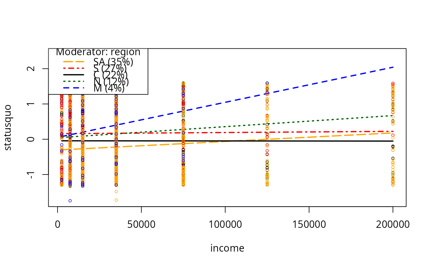 plotSlopes(m7, plotx = "income", modx = "region", plotPoints = FALSE)
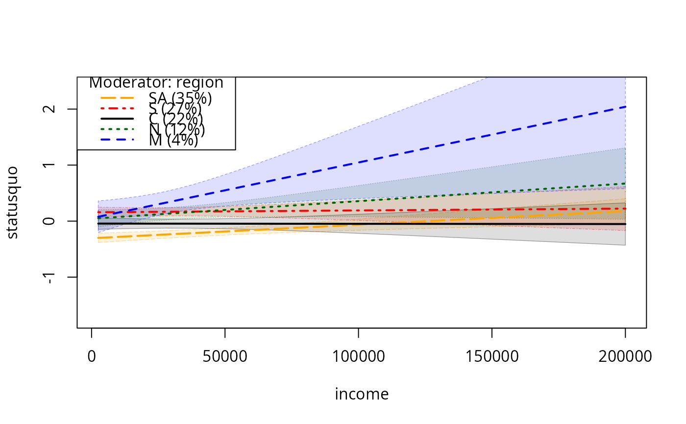
 plotSlopes(m7, plotx = "income", modx = "region", plotPoints = FALSE,
interval = "conf")
plotSlopes(m7, plotx = "income", modx = "region", plotPoints = FALSE,
interval = "conf")
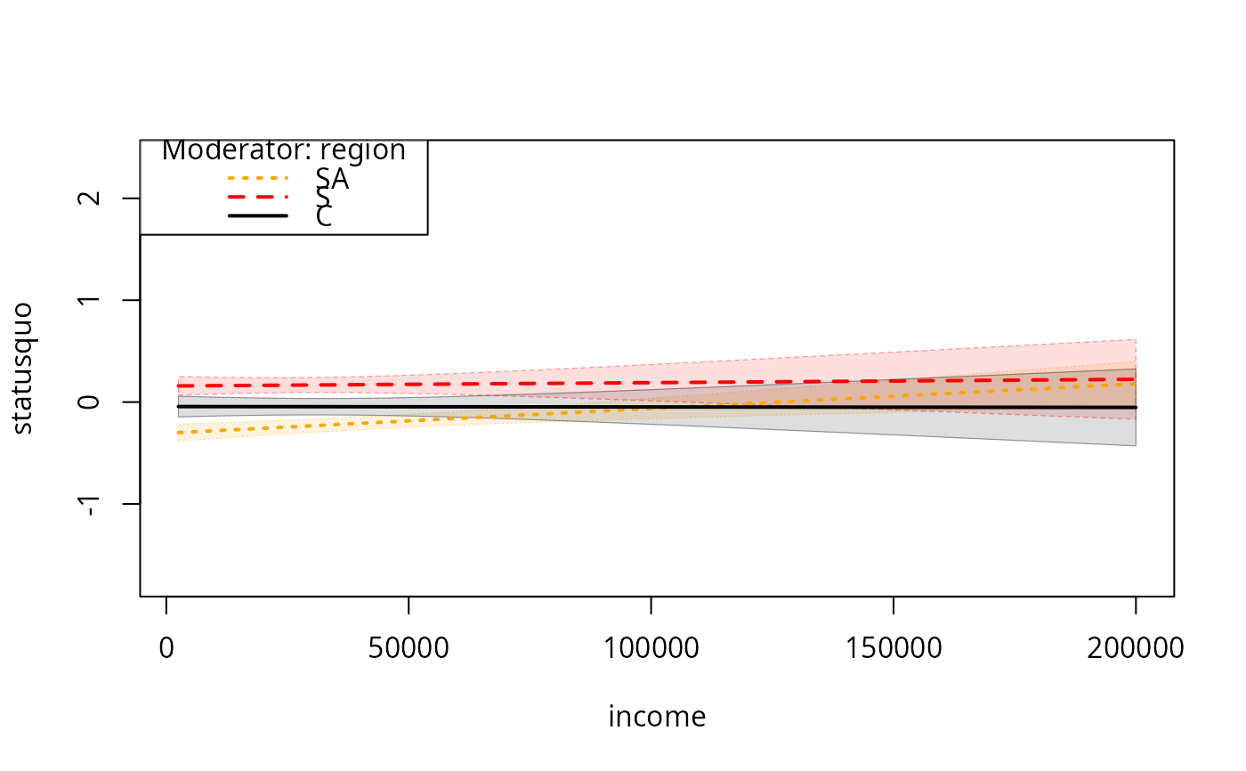
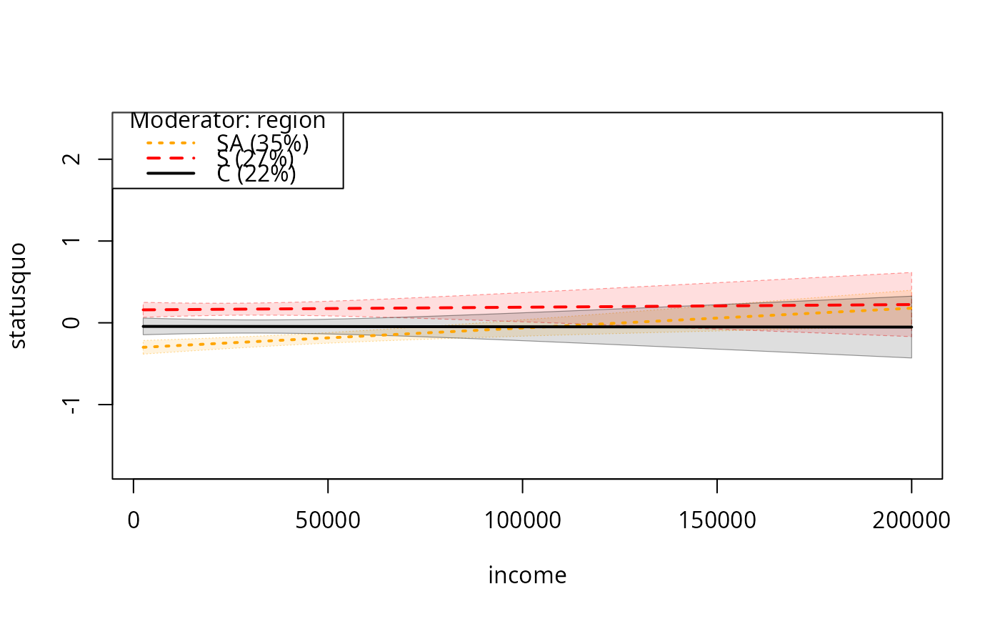
 plotSlopes(m7, plotx = "income", modx = "region", modxVals = c("SA","S", "C"),
plotPoints = FALSE, interval = "conf")
plotSlopes(m7, plotx = "income", modx = "region", modxVals = c("SA","S", "C"),
plotPoints = FALSE, interval = "conf")
 ## Same, choosing 3 most frequent values
plotSlopes(m7, plotx = "income", modx = "region", n = 3, plotPoints = FALSE,
interval = "conf")
## Same, choosing 3 most frequent values
plotSlopes(m7, plotx = "income", modx = "region", n = 3, plotPoints = FALSE,
interval = "conf")
 m8 <- lm(statusquo ~ region * income + sex + age, data= Chile)
summary(m8)
#>
#> Call:
#> lm(formula = statusquo ~ region * income + sex + age, data = Chile)
#>
#> Residuals:
#> Min 1Q Median 3Q Max
#> -1.75049 -0.90523 -0.05172 0.89764 1.90716
#>
#> Coefficients:
#> Estimate Std. Error t value Pr(>|t|)
#> (Intercept) -3.116e-01 7.539e-02 -4.133 3.69e-05 ***
#> regionM 9.231e-02 1.596e-01 0.578 0.56308
#> regionN 8.367e-02 9.580e-02 0.873 0.38251
#> regionS 2.097e-01 7.165e-02 2.926 0.00346 **
#> regionSA -2.732e-01 6.858e-02 -3.983 6.98e-05 ***
#> income 2.734e-07 1.106e-06 0.247 0.80475
#> sexM -1.509e-01 3.839e-02 -3.932 8.64e-05 ***
#> age 8.707e-03 1.307e-03 6.664 3.25e-11 ***
#> regionM:income 1.044e-05 4.350e-06 2.400 0.01648 *
#> regionN:income 3.042e-06 2.173e-06 1.400 0.16172
#> regionS:income 3.333e-07 1.575e-06 0.212 0.83244
#> regionSA:income 2.334e-06 1.295e-06 1.802 0.07160 .
#> ---
#> Signif. codes: 0 ‘***’ 0.001 ‘**’ 0.01 ‘*’ 0.05 ‘.’ 0.1 ‘ ’ 1
#>
#> Residual standard error: 0.9741 on 2578 degrees of freedom
#> (110 observations deleted due to missingness)
#> Multiple R-squared: 0.05727, Adjusted R-squared: 0.05324
#> F-statistic: 14.24 on 11 and 2578 DF, p-value: < 2.2e-16
#>
plotSlopes(m8, modx = "region", plotx = "income")
m8 <- lm(statusquo ~ region * income + sex + age, data= Chile)
summary(m8)
#>
#> Call:
#> lm(formula = statusquo ~ region * income + sex + age, data = Chile)
#>
#> Residuals:
#> Min 1Q Median 3Q Max
#> -1.75049 -0.90523 -0.05172 0.89764 1.90716
#>
#> Coefficients:
#> Estimate Std. Error t value Pr(>|t|)
#> (Intercept) -3.116e-01 7.539e-02 -4.133 3.69e-05 ***
#> regionM 9.231e-02 1.596e-01 0.578 0.56308
#> regionN 8.367e-02 9.580e-02 0.873 0.38251
#> regionS 2.097e-01 7.165e-02 2.926 0.00346 **
#> regionSA -2.732e-01 6.858e-02 -3.983 6.98e-05 ***
#> income 2.734e-07 1.106e-06 0.247 0.80475
#> sexM -1.509e-01 3.839e-02 -3.932 8.64e-05 ***
#> age 8.707e-03 1.307e-03 6.664 3.25e-11 ***
#> regionM:income 1.044e-05 4.350e-06 2.400 0.01648 *
#> regionN:income 3.042e-06 2.173e-06 1.400 0.16172
#> regionS:income 3.333e-07 1.575e-06 0.212 0.83244
#> regionSA:income 2.334e-06 1.295e-06 1.802 0.07160 .
#> ---
#> Signif. codes: 0 ‘***’ 0.001 ‘**’ 0.01 ‘*’ 0.05 ‘.’ 0.1 ‘ ’ 1
#>
#> Residual standard error: 0.9741 on 2578 degrees of freedom
#> (110 observations deleted due to missingness)
#> Multiple R-squared: 0.05727, Adjusted R-squared: 0.05324
#> F-statistic: 14.24 on 11 and 2578 DF, p-value: < 2.2e-16
#>
plotSlopes(m8, modx = "region", plotx = "income")
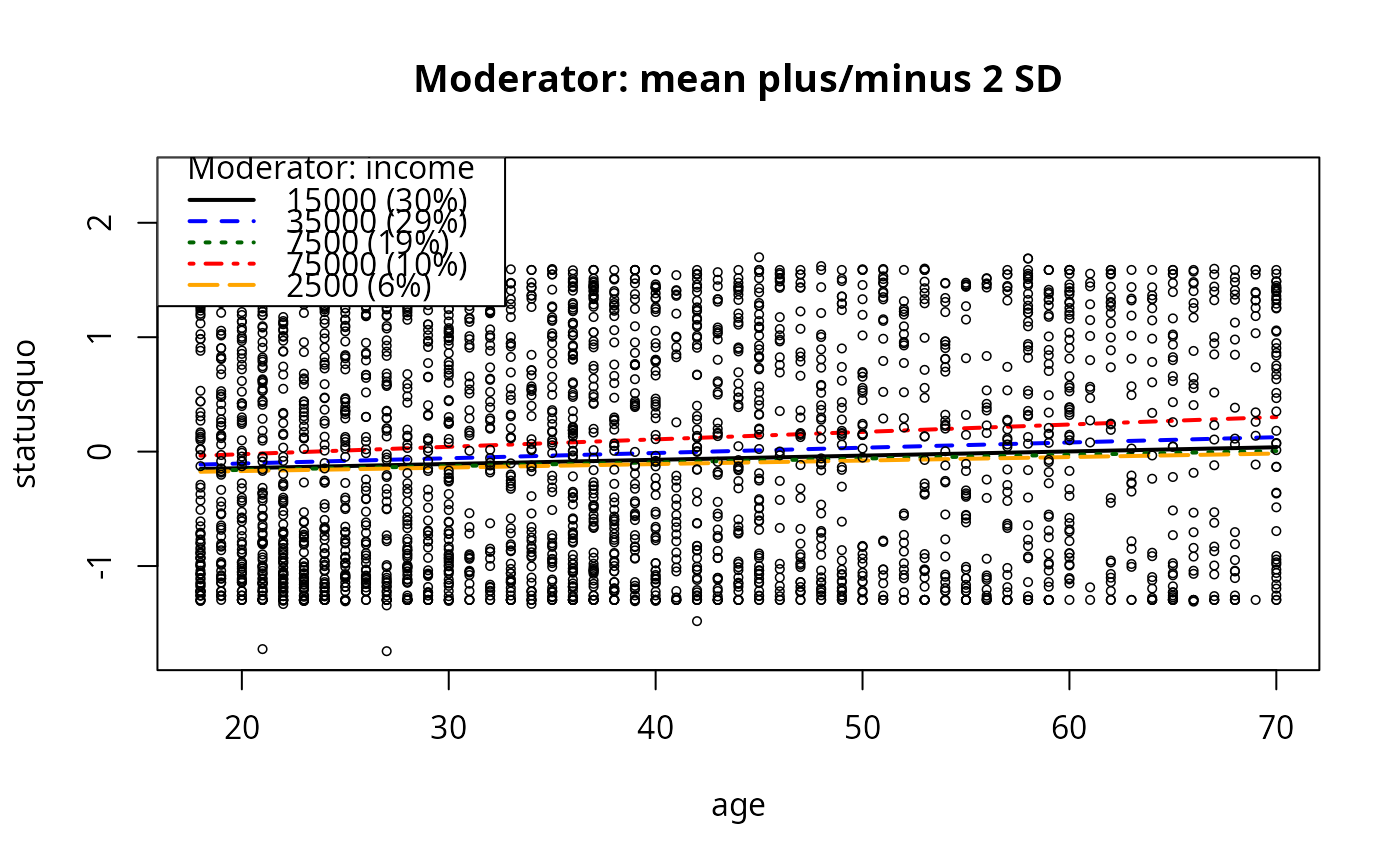
 m9 <- lm(statusquo ~ income * age + education + sex + age, data = Chile)
summary(m9)
#>
#> Call:
#> lm(formula = statusquo ~ income * age + education + sex + age,
#> data = Chile)
#>
#> Residuals:
#> Min 1Q Median 3Q Max
#> -1.72763 -0.91292 -0.07841 0.93242 2.04934
#>
#> Coefficients:
#> Estimate Std. Error t value Pr(>|t|)
#> (Intercept) 2.413e-02 8.567e-02 0.282 0.77827
#> income 1.088e-06 1.476e-06 0.737 0.46089
#> age 2.943e-03 1.837e-03 1.602 0.10928
#> educationPS -4.474e-01 6.478e-02 -6.906 6.27e-12 ***
#> educationS -2.581e-01 4.656e-02 -5.543 3.28e-08 ***
#> sexM -1.224e-01 3.886e-02 -3.150 0.00165 **
#> income:age 4.726e-08 3.587e-08 1.318 0.18775
#> ---
#> Signif. codes: 0 ‘***’ 0.001 ‘**’ 0.01 ‘*’ 0.05 ‘.’ 0.1 ‘ ’ 1
#>
#> Residual standard error: 0.9818 on 2574 degrees of freedom
#> (119 observations deleted due to missingness)
#> Multiple R-squared: 0.04021, Adjusted R-squared: 0.03797
#> F-statistic: 17.97 on 6 and 2574 DF, p-value: < 2.2e-16
#>
plotSlopes(m9, modx = "income", plotx = "age")
m9 <- lm(statusquo ~ income * age + education + sex + age, data = Chile)
summary(m9)
#>
#> Call:
#> lm(formula = statusquo ~ income * age + education + sex + age,
#> data = Chile)
#>
#> Residuals:
#> Min 1Q Median 3Q Max
#> -1.72763 -0.91292 -0.07841 0.93242 2.04934
#>
#> Coefficients:
#> Estimate Std. Error t value Pr(>|t|)
#> (Intercept) 2.413e-02 8.567e-02 0.282 0.77827
#> income 1.088e-06 1.476e-06 0.737 0.46089
#> age 2.943e-03 1.837e-03 1.602 0.10928
#> educationPS -4.474e-01 6.478e-02 -6.906 6.27e-12 ***
#> educationS -2.581e-01 4.656e-02 -5.543 3.28e-08 ***
#> sexM -1.224e-01 3.886e-02 -3.150 0.00165 **
#> income:age 4.726e-08 3.587e-08 1.318 0.18775
#> ---
#> Signif. codes: 0 ‘***’ 0.001 ‘**’ 0.01 ‘*’ 0.05 ‘.’ 0.1 ‘ ’ 1
#>
#> Residual standard error: 0.9818 on 2574 degrees of freedom
#> (119 observations deleted due to missingness)
#> Multiple R-squared: 0.04021, Adjusted R-squared: 0.03797
#> F-statistic: 17.97 on 6 and 2574 DF, p-value: < 2.2e-16
#>
plotSlopes(m9, modx = "income", plotx = "age")
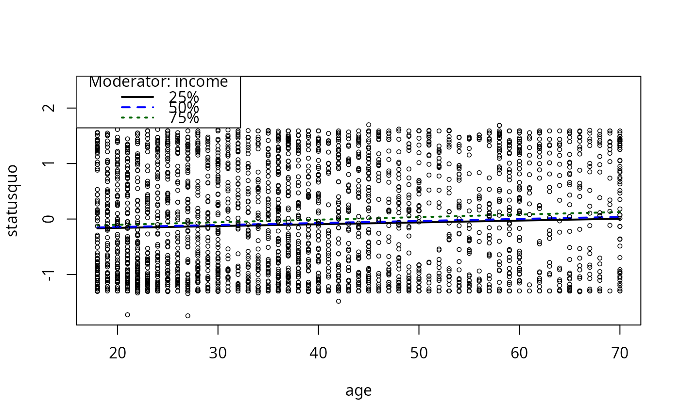 m9ps <- plotSlopes(m9, modx = "income", plotx = "age")
m9psts <- testSlopes(m9ps)
#> Error in eval(parse(text = object$call$model)): object 'm9' not found
plot(m9psts) ## only works if moderator is numeric
#> Error: object 'm9psts' not found
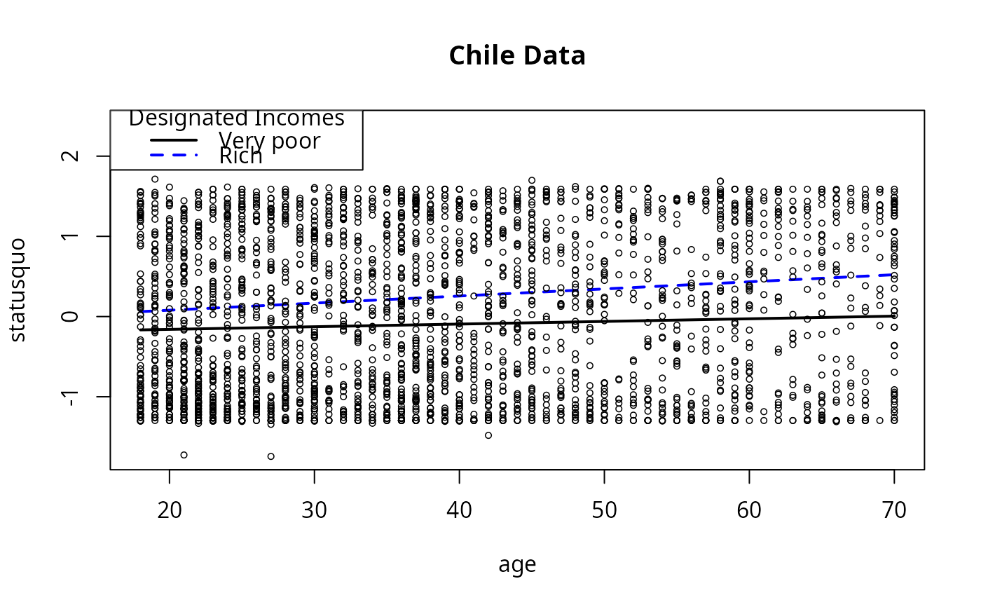
## Demonstrate re-labeling
plotSlopes(m9, modx = "income", plotx = "age", n = 5,
modxVals = c("Very poor" = 7500, "Rich" = 125000),
main = "Chile Data", legendArgs = list(title = "Designated Incomes"))
m9ps <- plotSlopes(m9, modx = "income", plotx = "age")
m9psts <- testSlopes(m9ps)
#> Error in eval(parse(text = object$call$model)): object 'm9' not found
plot(m9psts) ## only works if moderator is numeric
#> Error: object 'm9psts' not found
## Demonstrate re-labeling
plotSlopes(m9, modx = "income", plotx = "age", n = 5,
modxVals = c("Very poor" = 7500, "Rich" = 125000),
main = "Chile Data", legendArgs = list(title = "Designated Incomes"))
 plotSlopes(m9, modx = "income", plotx = "age", n = 5, modxVals = c("table"),
main = "Moderator: mean plus/minus 2 SD")
plotSlopes(m9, modx = "income", plotx = "age", n = 5, modxVals = c("table"),
main = "Moderator: mean plus/minus 2 SD")
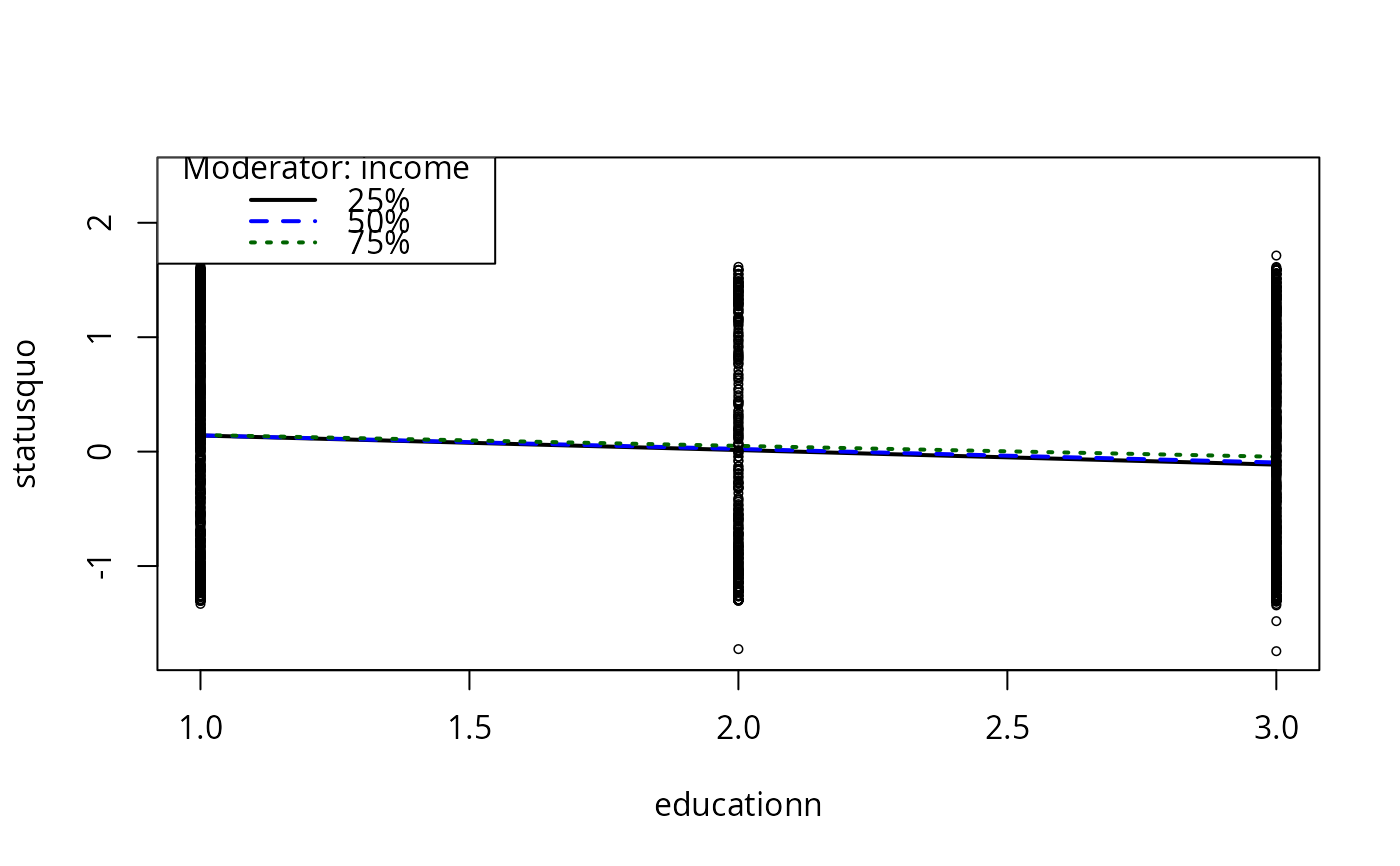
 ## Convert education to numeric, for fun
Chile$educationn <- as.numeric(Chile$education)
m10 <- lm(statusquo ~ income * educationn + sex + age, data = Chile)
summary(m10)
#>
#> Call:
#> lm(formula = statusquo ~ income * educationn + sex + age, data = Chile)
#>
#> Residuals:
#> Min 1Q Median 3Q Max
#> -1.67568 -0.93318 -0.06687 0.95047 2.05457
#>
#> Coefficients:
#> Estimate Std. Error t value Pr(>|t|)
#> (Intercept) 5.480e-02 9.491e-02 0.577 0.563749
#> income -9.986e-07 1.852e-06 -0.539 0.589722
#> educationn -1.361e-01 3.058e-02 -4.449 9.01e-06 ***
#> sexM -1.341e-01 3.901e-02 -3.437 0.000598 ***
#> age 5.732e-03 1.402e-03 4.088 4.49e-05 ***
#> income:educationn 1.166e-06 7.956e-07 1.466 0.142816
#> ---
#> Signif. codes: 0 ‘***’ 0.001 ‘**’ 0.01 ‘*’ 0.05 ‘.’ 0.1 ‘ ’ 1
#>
#> Residual standard error: 0.9875 on 2575 degrees of freedom
#> (119 observations deleted due to missingness)
#> Multiple R-squared: 0.02859, Adjusted R-squared: 0.02671
#> F-statistic: 15.16 on 5 and 2575 DF, p-value: 1.054e-14
#>
plotSlopes(m10, plotx = "educationn", modx = "income")
## Convert education to numeric, for fun
Chile$educationn <- as.numeric(Chile$education)
m10 <- lm(statusquo ~ income * educationn + sex + age, data = Chile)
summary(m10)
#>
#> Call:
#> lm(formula = statusquo ~ income * educationn + sex + age, data = Chile)
#>
#> Residuals:
#> Min 1Q Median 3Q Max
#> -1.67568 -0.93318 -0.06687 0.95047 2.05457
#>
#> Coefficients:
#> Estimate Std. Error t value Pr(>|t|)
#> (Intercept) 5.480e-02 9.491e-02 0.577 0.563749
#> income -9.986e-07 1.852e-06 -0.539 0.589722
#> educationn -1.361e-01 3.058e-02 -4.449 9.01e-06 ***
#> sexM -1.341e-01 3.901e-02 -3.437 0.000598 ***
#> age 5.732e-03 1.402e-03 4.088 4.49e-05 ***
#> income:educationn 1.166e-06 7.956e-07 1.466 0.142816
#> ---
#> Signif. codes: 0 ‘***’ 0.001 ‘**’ 0.01 ‘*’ 0.05 ‘.’ 0.1 ‘ ’ 1
#>
#> Residual standard error: 0.9875 on 2575 degrees of freedom
#> (119 observations deleted due to missingness)
#> Multiple R-squared: 0.02859, Adjusted R-squared: 0.02671
#> F-statistic: 15.16 on 5 and 2575 DF, p-value: 1.054e-14
#>
plotSlopes(m10, plotx = "educationn", modx = "income")
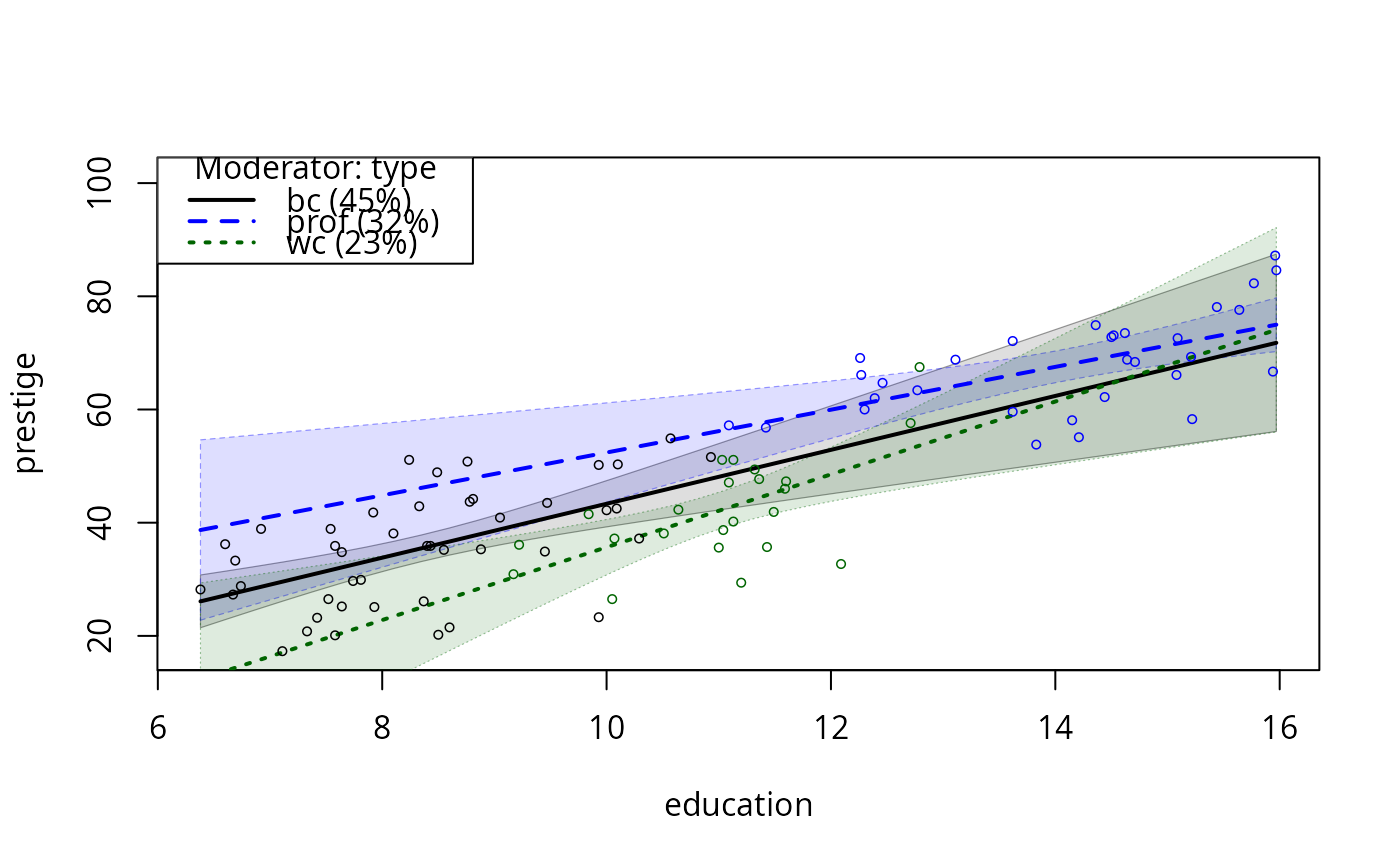
 ## Now, the occupational prestige data. Please note careful attention
## to consistency of colors selected
data(Prestige)
m11 <- lm(prestige ~ education * type, data = Prestige)
plotSlopes(m11, plotx = "education", modx = "type", interval = "conf")
## Now, the occupational prestige data. Please note careful attention
## to consistency of colors selected
data(Prestige)
m11 <- lm(prestige ~ education * type, data = Prestige)
plotSlopes(m11, plotx = "education", modx = "type", interval = "conf")
 dev.new()
plotSlopes(m11, plotx = "education", modx = "type",
modxVals = c("prof"), interval = "conf")
dev.new()
plotSlopes(m11, plotx = "education", modx = "type",
modxVals = c("bc"), interval = "conf")
dev.new()
plotSlopes(m11, plotx = "education", modx = "type",
modxVals = c("bc", "wc"), interval = "conf")
dev.new()
plotSlopes(m11, plotx = "education", modx = "type",
modxVals = c("prof"), interval = "conf")
dev.new()
plotSlopes(m11, plotx = "education", modx = "type",
modxVals = c("bc"), interval = "conf")
dev.new()
plotSlopes(m11, plotx = "education", modx = "type",
modxVals = c("bc", "wc"), interval = "conf")