Assists creation of predicted value curves for regression models.
plotCurves.RdCreates a predicted value plot that includes a separate predicted
value line for each value of a focal variable. The x axis variable
is specified by the plotx argument. As of rockchalk 1.7.x,
the moderator argument, modx, is optional. Think of this a new
version of R's termplot, but it allows for
interactions. And it handles some nonlinear transformations more
gracefully than termplot.
Usage
plotCurves(
  model,
  plotx,
  nx = 40,
  modx,
  plotxRange = NULL,
  n,
  modxVals = NULL,
  interval = c("none", "confidence", "prediction"),
  plotPoints = TRUE,
  plotLegend = TRUE,
  legendTitle = NULL,
  legendPct = TRUE,
  col = c("black", "blue", "darkgreen", "red", "orange", "purple", "green3"),
  llwd = 2,
  opacity = 100,
  envir = environment(formula(model)),
  ...
)
Arguments
- model
Required. Fitted regression object. Must have a predict method
- plotx
Required. String with name of predictor for the x axis
- nx
Number of values of plotx at which to calculate the predicted value. Default = 40.
- modx
Optional. String for moderator variable name. May be either numeric or factor.
- plotxRange
Optional. If not specified, the observed range of plotx will be used to determine the axis range.
- n
Optional. Number of focal values of
modx, used by algorithms specified by modxVals; will be ignored if modxVals supplies a vector of focal values.- modxVals
Optional. A vector of focal values for which predicted values are to be plotted. May also be a character string to select an algorithm ("quantile","std.dev." or "table"), or a user-supplied function to select focal values (a new method similar to
getFocal). If modx is a factor, currently, the only available algorithm is "table" (seegetFocal.factor.- interval
Optional. Intervals provided by the
predict.lmmay be supplied, either "conf" (95 interval for the estimated conditional mean) or "pred" (95 interval for observed values of y given the rest of the model).- plotPoints
Optional. TRUE or FALSE: Should the plot include the scatterplot points along with the lines.
- plotLegend
Optional. TRUE or FALSE: Should the default legend be included?
- legendTitle
Optional. You'll get an automatically generated title, such as "Moderator: modx", but if you don't like that, specify your own string here.
- legendPct
Default = TRUE. Variable labels print with sample percentages.
- col
I offer my preferred color vector as default. Replace if you like. User may supply a vector of valid color names, or
rainbow(10)orgray.colors(5). Color names will be recycled if there are more focal values ofmodxthan colors provided.- llwd
Optional. Line widths for predicted values. Can be single value or a vector, which will be recycled as necessary.
- opacity
Optional, default = 100. A number between 1 and 255. 1 means "transparent" or invisible, 255 means very dark. the darkness of confidence interval regions
- envir
environment to search for variables.
- ...
further arguments that are passed to plot or predict. The arguments that are monitored to be sent to predict are c("type", "se.fit", "dispersion", "interval", "level", "terms", "na.action").
Value
A plot is created as a side effect, a list is returned including 1) the call, 2) a newdata object that includes information on the curves that were plotted, 3) a vector modxVals, the values for which curves were drawn.
Details
This is similar to plotSlopes, but it accepts regressions
in which there are transformed variables, such as "log(x1)".
It creates a plot of the predicted dependent
variable against one of the numeric predictors, plotx. It
draws a predicted value line for each value of modx, a
moderator variable. The moderator may be a numeric or categorical
moderator variable.
The user may designate which particular values of the moderator
are used for calculating the predicted value lines. That is,
modxVals = c( 12,22,37) would draw lines for values 12, 22,
and 37 of the moderator. User may instead supply a character
string to choose one of the built in algorithms. The default
algorithm is "quantile", which will select n values that
are evenly spaced along the modx axis. The algorithm
"std.dev" will select the mean of modx (m) and then it will
select values that step away from the mean in standard deviation
sd units. For example, if n = 3, the focal
values will m, m - sd, am + sd.
Author
Paul E. Johnson pauljohn@ku.edu
Examples
library(rockchalk)
## Replicate some R classics. The budworm.lg data from predict.glm
## will work properly after re-formatting the information as a data.frame:
## example from Venables and Ripley (2002, pp. 190-2.)
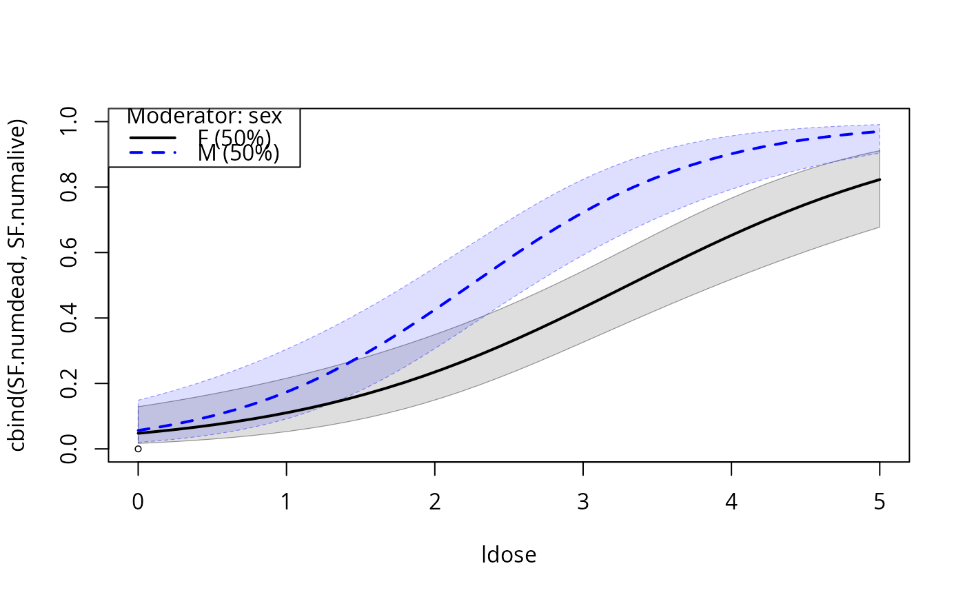
df <- data.frame(ldose = rep(0:5, 2),
sex = factor(rep(c("M", "F"), c(6, 6))),
SF.numdead = c(1, 4, 9, 13, 18, 20, 0, 2, 6, 10, 12, 16))
df$SF.numalive = 20 - df$SF.numdead
budworm.lg <- glm(cbind(SF.numdead, SF.numalive) ~ sex*ldose, data = df,
family = binomial)
plotCurves(budworm.lg, plotx = "ldose", modx = "sex", interval = "confidence",
ylim = c(0, 1))
#> Warning: Using formula(x) is deprecated when x is a character vector of length > 1.
#> Consider formula(paste(x, collapse = " ")) instead.
#> rockchalk:::predCI: model's predict method does not return an interval.
#> We will improvize with a Wald type approximation to the confidence interval
#> Warning: no non-missing arguments to min; returning Inf
#> Warning: no non-missing arguments to max; returning -Inf
 ## See infert
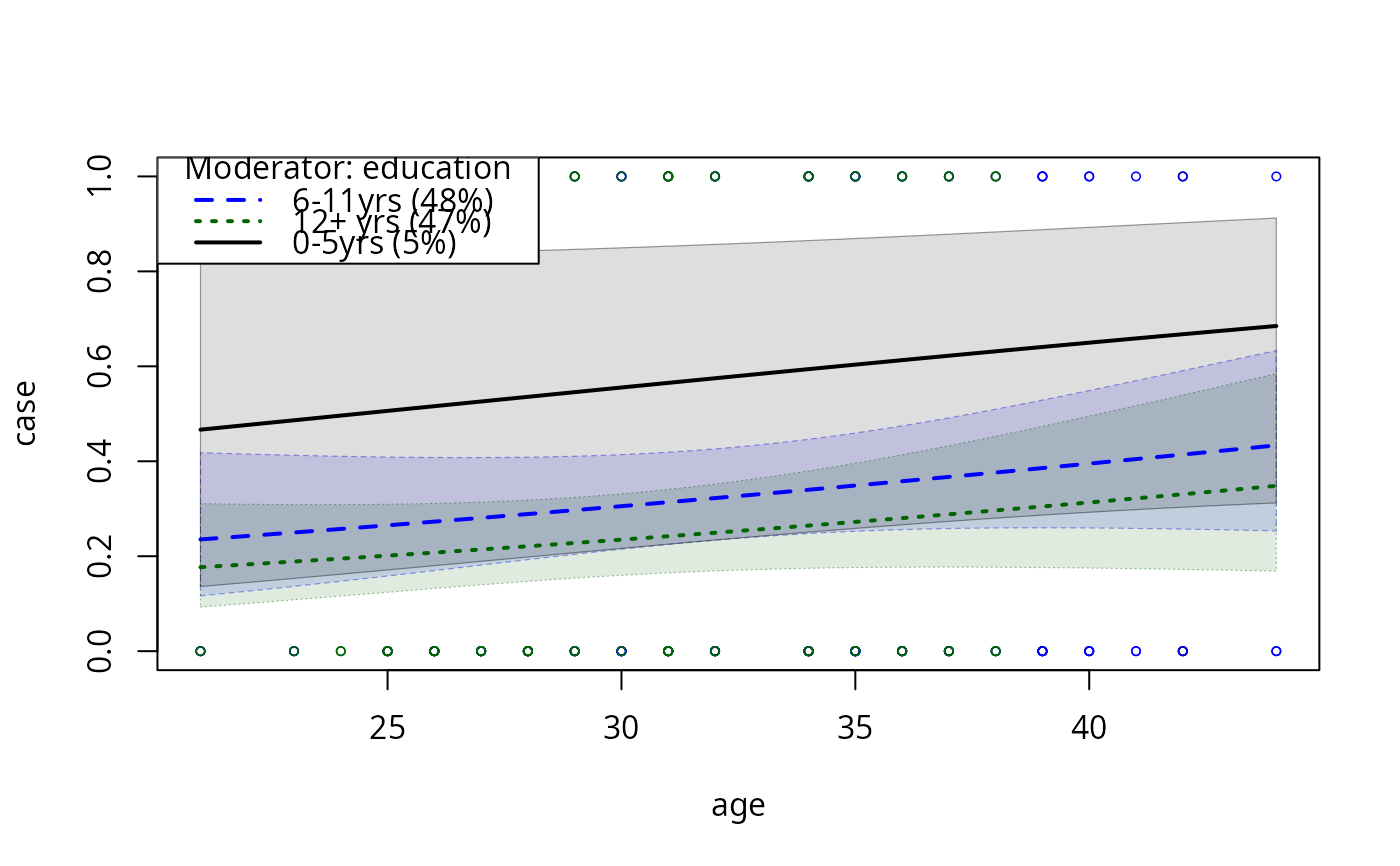
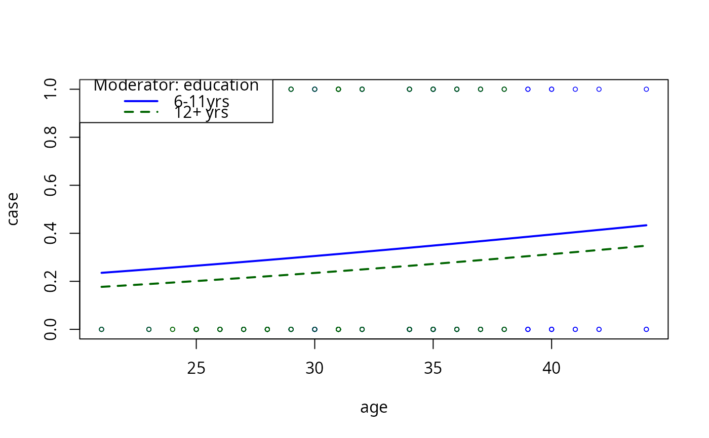
model2 <- glm(case ~ age + parity + education + spontaneous + induced,
data = infert, family = binomial())
## Curvature so slight we can barely see it
model2pc1 <- plotCurves(model2, plotx = "age", modx = "education",
interval = "confidence", ylim = c(0, 1))
#> rockchalk:::predCI: model's predict method does not return an interval.
#> We will improvize with a Wald type approximation to the confidence interval
## See infert
model2 <- glm(case ~ age + parity + education + spontaneous + induced,
data = infert, family = binomial())
## Curvature so slight we can barely see it
model2pc1 <- plotCurves(model2, plotx = "age", modx = "education",
interval = "confidence", ylim = c(0, 1))
#> rockchalk:::predCI: model's predict method does not return an interval.
#> We will improvize with a Wald type approximation to the confidence interval
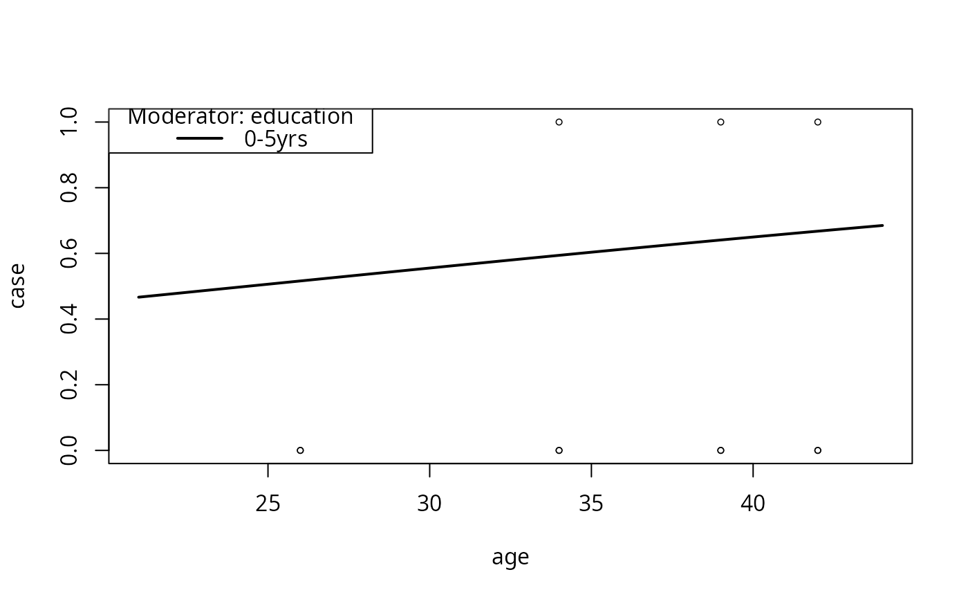
 model2pc2 <- plotCurves(model2, plotx = "age", modx = "education",
modxVals = levels(infert$education)[1],
interval = "confidence", ylim = c(0, 1))
#> rockchalk:::predCI: model's predict method does not return an interval.
#> We will improvize with a Wald type approximation to the confidence interval
model2pc2 <- plotCurves(model2, plotx = "age", modx = "education",
modxVals = levels(infert$education)[1],
interval = "confidence", ylim = c(0, 1))
#> rockchalk:::predCI: model's predict method does not return an interval.
#> We will improvize with a Wald type approximation to the confidence interval
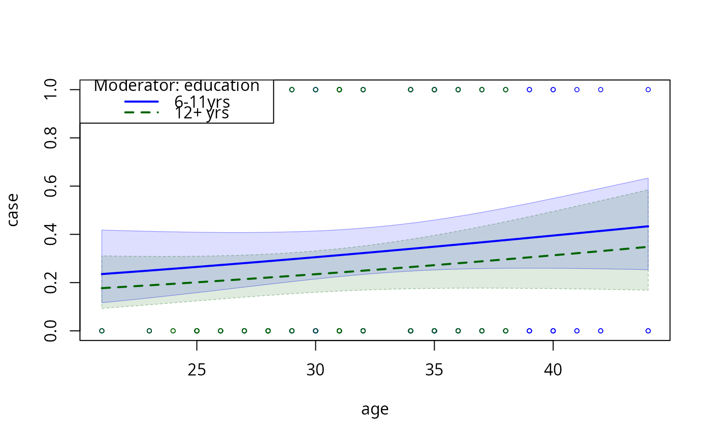
 model2pc2 <- plotCurves(model2, plotx = "age", modx = "education",
modxVals = levels(infert$education)[c(2,3)],
interval = "confidence", ylim = c(0, 1))
#> rockchalk:::predCI: model's predict method does not return an interval.
#> We will improvize with a Wald type approximation to the confidence interval
model2pc2 <- plotCurves(model2, plotx = "age", modx = "education",
modxVals = levels(infert$education)[c(2,3)],
interval = "confidence", ylim = c(0, 1))
#> rockchalk:::predCI: model's predict method does not return an interval.
#> We will improvize with a Wald type approximation to the confidence interval
 model2pc2 <- plotCurves(model2, plotx = "age", modx = "education",
modxVals = levels(infert$education)[c(2,3)],
ylim = c(0, 1), type = "response")
model2pc2 <- plotCurves(model2, plotx = "age", modx = "education",
modxVals = levels(infert$education)[c(2,3)],
ylim = c(0, 1), type = "response")
 ## Manufacture some data
set.seed(12345)
N <- 500
dat <- genCorrelatedData2(N = 500, means = c(5, 0, 0, 0), sds = rep(1, 4),
rho = 0.2, beta = rep(1, 5), stde = 20)
#> [1] "The equation that was calculated was"
#> y = 1 + 1*x1 + 1*x2 + 1*x3 + 1*x4
#> + 0*x1*x1 + 0*x2*x1 + 0*x3*x1 + 0*x4*x1
#> + 0*x1*x2 + 0*x2*x2 + 0*x3*x2 + 0*x4*x2
#> + 0*x1*x3 + 0*x2*x3 + 0*x3*x3 + 0*x4*x3
#> + 0*x1*x4 + 0*x2*x4 + 0*x3*x4 + 0*x4*x4
#> + N(0,20) random error
dat$xcat1 <- gl(2, N/2, labels = c("Monster", "Human"))
dat$xcat2 <- cut(rnorm(N), breaks = c(-Inf, 0, 0.4, 0.9, 1, Inf),
labels = c("R", "M", "D", "P", "G"))
###The design matrix for categorical variables, xcat numeric
dat$xcat1n <- with(dat, contrasts(xcat1)[xcat1, ])
dat$xcat2n <- with(dat, contrasts(xcat2)[xcat2, ])
stde <- 2
dat$y <- with(dat, 0.03 + 11.5 * log(x1) * contrasts(dat$xcat1)[dat$xcat1] +
0.1 * x2 + 0.04 * x2^2 + stde*rnorm(N))
stde <- 1
dat$y2 <- with(dat, 0.03 + 0.1 * x1 + 0.1 * x2 + 0.25 * x1 * x2 + 0.4 * x3 -
0.1 * x4 + stde * rnorm(N))
stde <- 8
dat$y3 <- with(dat, 3 + 0.5 * x1 + 1.2 * (as.numeric(xcat1)-1) +
-0.8 * (as.numeric(xcat1)-1) * x1 + stde * rnorm(N))
stde <- 8
dat$y4 <- with(dat, 3 + 0.5 * x1 +
contrasts(dat$xcat2)[dat$xcat2, ] %*% c(0.1, -0.2, 0.3, 0.05) +
stde * rnorm(N))
## Curvature with interaction
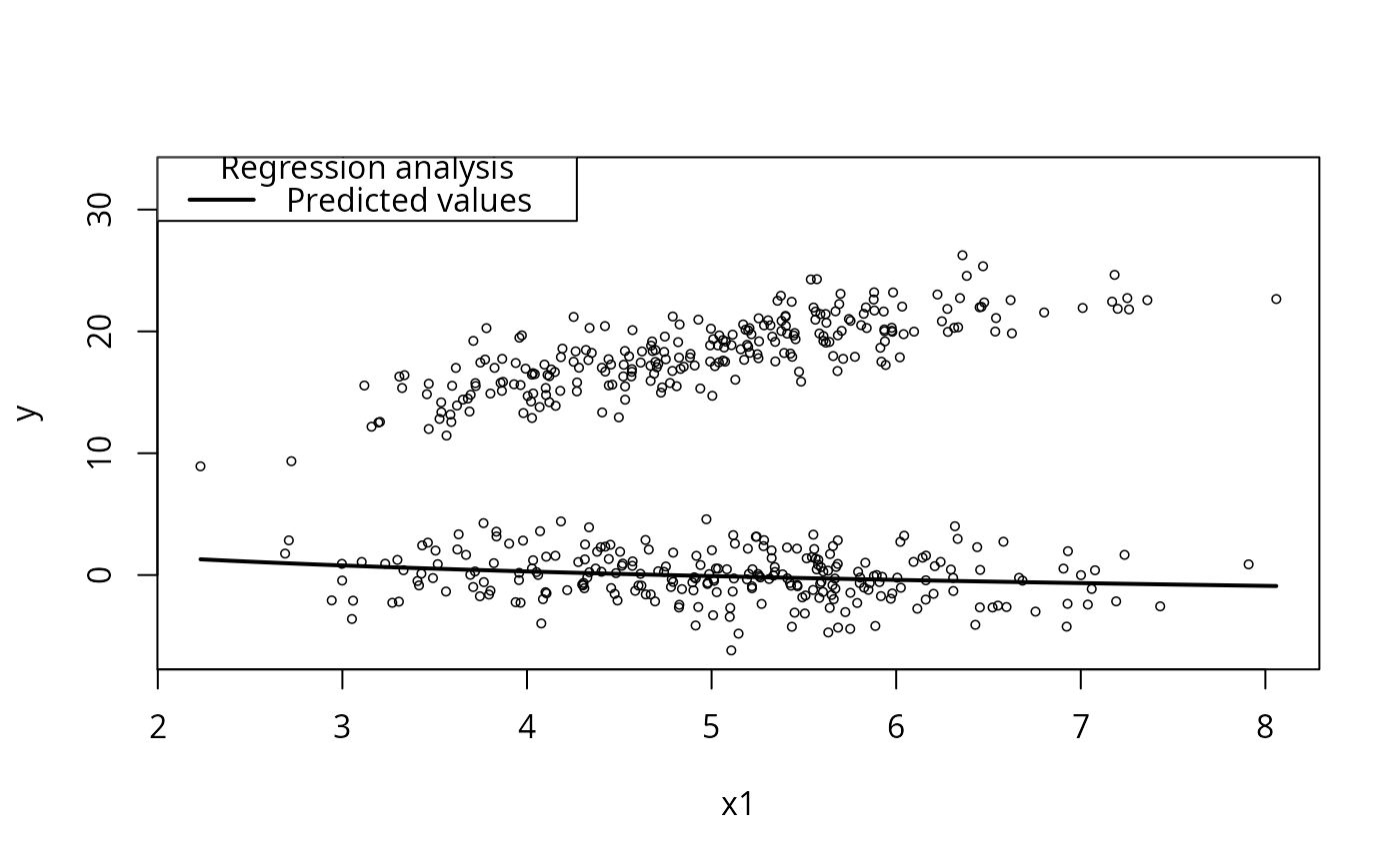
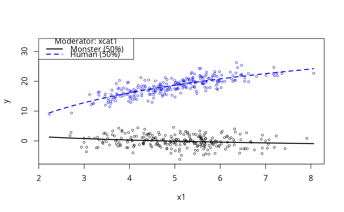
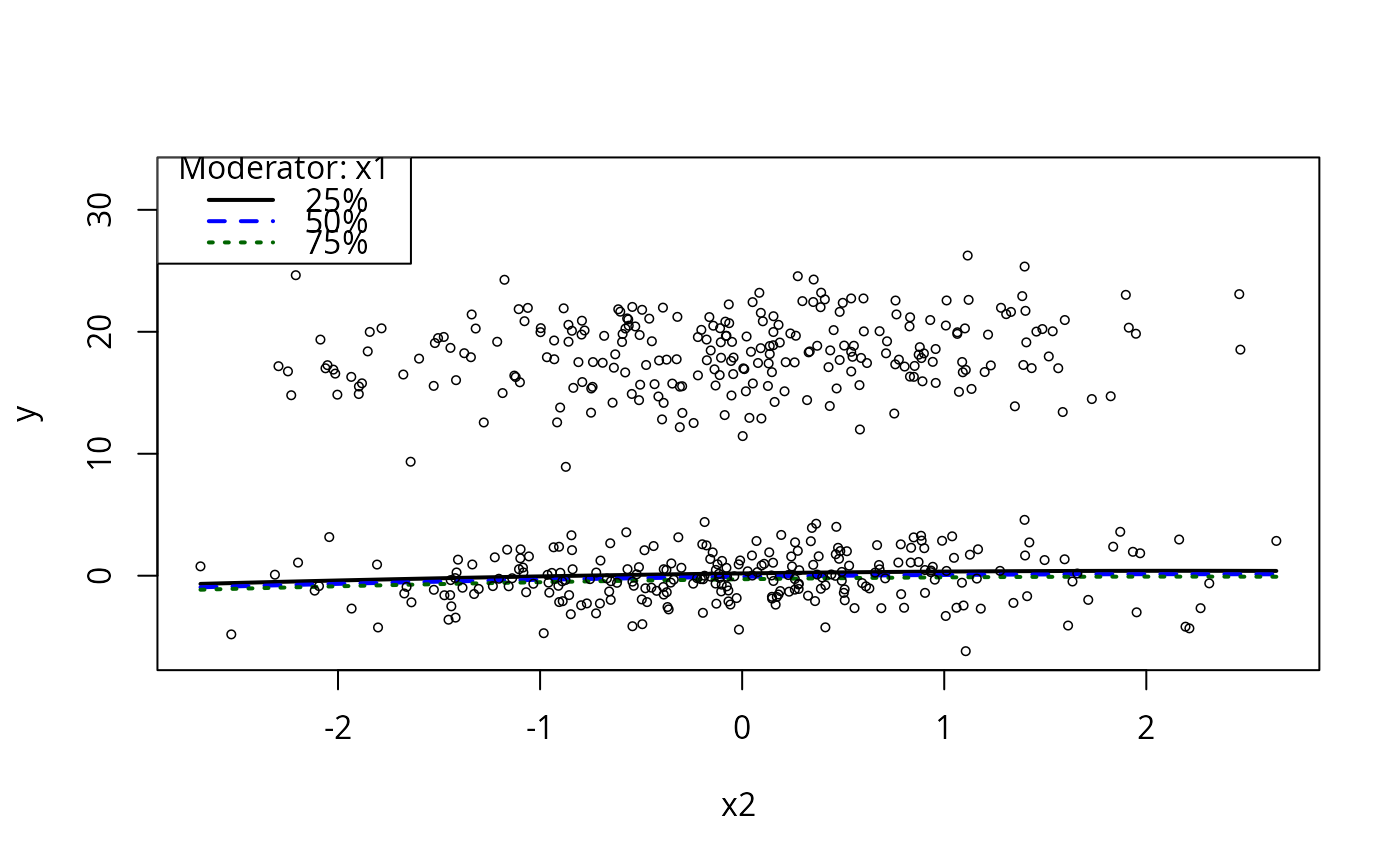
m1 <- lm(y ~ log(x1)*xcat1 + x2 + I(x2^2), data=dat)
summary(m1)
#>
#> Call:
#> lm(formula = y ~ log(x1) * xcat1 + x2 + I(x2^2), data = dat)
#>
#> Residuals:
#> Min 1Q Median 3Q Max
#> -6.2368 -1.2216 -0.0446 1.2399 4.9315
#>
#> Coefficients:
#> Estimate Std. Error t value Pr(>|t|)
#> (Intercept) 2.67164 0.91475 2.921 0.00365 **
#> log(x1) -1.70802 0.56807 -3.007 0.00278 **
#> xcat1Human -2.51612 1.29846 -1.938 0.05322 .
#> x2 0.19792 0.08673 2.282 0.02290 *
#> I(x2^2) -0.04577 0.06426 -0.712 0.47670
#> log(x1):xcat1Human 13.21959 0.81000 16.320 < 2e-16 ***
#> ---
#> Signif. codes: 0 ‘***’ 0.001 ‘**’ 0.01 ‘*’ 0.05 ‘.’ 0.1 ‘ ’ 1
#>
#> Residual standard error: 1.857 on 494 degrees of freedom
#> Multiple R-squared: 0.9626, Adjusted R-squared: 0.9622
#> F-statistic: 2542 on 5 and 494 DF, p-value: < 2.2e-16
#>
## First, with no moderator
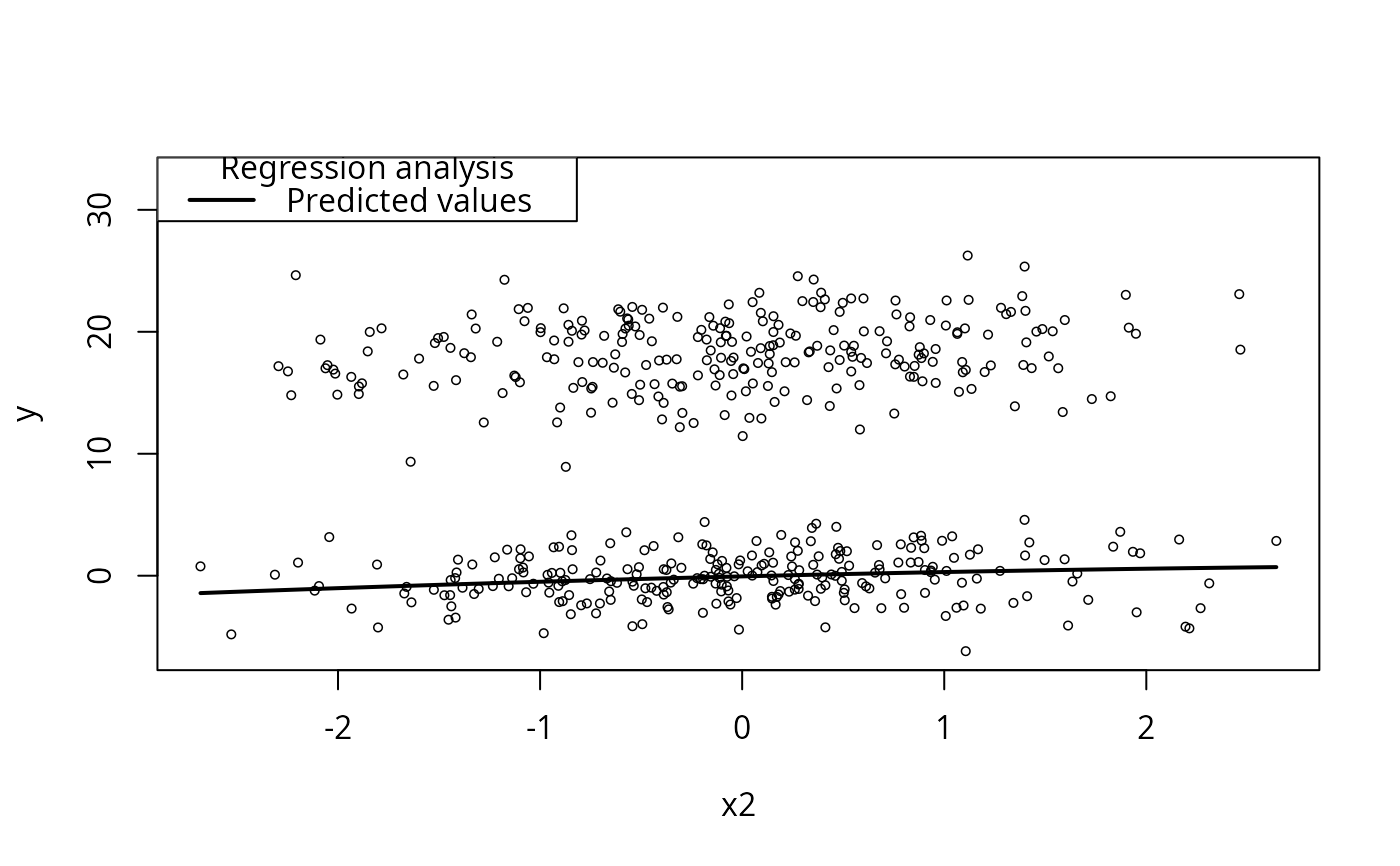
plotCurves(m1, plotx = "x1")
## Manufacture some data
set.seed(12345)
N <- 500
dat <- genCorrelatedData2(N = 500, means = c(5, 0, 0, 0), sds = rep(1, 4),
rho = 0.2, beta = rep(1, 5), stde = 20)
#> [1] "The equation that was calculated was"
#> y = 1 + 1*x1 + 1*x2 + 1*x3 + 1*x4
#> + 0*x1*x1 + 0*x2*x1 + 0*x3*x1 + 0*x4*x1
#> + 0*x1*x2 + 0*x2*x2 + 0*x3*x2 + 0*x4*x2
#> + 0*x1*x3 + 0*x2*x3 + 0*x3*x3 + 0*x4*x3
#> + 0*x1*x4 + 0*x2*x4 + 0*x3*x4 + 0*x4*x4
#> + N(0,20) random error
dat$xcat1 <- gl(2, N/2, labels = c("Monster", "Human"))
dat$xcat2 <- cut(rnorm(N), breaks = c(-Inf, 0, 0.4, 0.9, 1, Inf),
labels = c("R", "M", "D", "P", "G"))
###The design matrix for categorical variables, xcat numeric
dat$xcat1n <- with(dat, contrasts(xcat1)[xcat1, ])
dat$xcat2n <- with(dat, contrasts(xcat2)[xcat2, ])
stde <- 2
dat$y <- with(dat, 0.03 + 11.5 * log(x1) * contrasts(dat$xcat1)[dat$xcat1] +
0.1 * x2 + 0.04 * x2^2 + stde*rnorm(N))
stde <- 1
dat$y2 <- with(dat, 0.03 + 0.1 * x1 + 0.1 * x2 + 0.25 * x1 * x2 + 0.4 * x3 -
0.1 * x4 + stde * rnorm(N))
stde <- 8
dat$y3 <- with(dat, 3 + 0.5 * x1 + 1.2 * (as.numeric(xcat1)-1) +
-0.8 * (as.numeric(xcat1)-1) * x1 + stde * rnorm(N))
stde <- 8
dat$y4 <- with(dat, 3 + 0.5 * x1 +
contrasts(dat$xcat2)[dat$xcat2, ] %*% c(0.1, -0.2, 0.3, 0.05) +
stde * rnorm(N))
## Curvature with interaction
m1 <- lm(y ~ log(x1)*xcat1 + x2 + I(x2^2), data=dat)
summary(m1)
#>
#> Call:
#> lm(formula = y ~ log(x1) * xcat1 + x2 + I(x2^2), data = dat)
#>
#> Residuals:
#> Min 1Q Median 3Q Max
#> -6.2368 -1.2216 -0.0446 1.2399 4.9315
#>
#> Coefficients:
#> Estimate Std. Error t value Pr(>|t|)
#> (Intercept) 2.67164 0.91475 2.921 0.00365 **
#> log(x1) -1.70802 0.56807 -3.007 0.00278 **
#> xcat1Human -2.51612 1.29846 -1.938 0.05322 .
#> x2 0.19792 0.08673 2.282 0.02290 *
#> I(x2^2) -0.04577 0.06426 -0.712 0.47670
#> log(x1):xcat1Human 13.21959 0.81000 16.320 < 2e-16 ***
#> ---
#> Signif. codes: 0 ‘***’ 0.001 ‘**’ 0.01 ‘*’ 0.05 ‘.’ 0.1 ‘ ’ 1
#>
#> Residual standard error: 1.857 on 494 degrees of freedom
#> Multiple R-squared: 0.9626, Adjusted R-squared: 0.9622
#> F-statistic: 2542 on 5 and 494 DF, p-value: < 2.2e-16
#>
## First, with no moderator
plotCurves(m1, plotx = "x1")
 plotCurves(m1, plotx = "x1", modx = "xcat1")
 ## ## Verify that plot by comparing against a manually contructed alternative
## par(mfrow=c(1,2))
## plotCurves(m1, plotx = "x1", modx = "xcat1")
## newdat <- with(dat, expand.grid(x1 = plotSeq(x1, 30), xcat1 = levels(xcat1)))
## newdat$x2 <- with(dat, mean(x2, na.rm = TRUE))
## newdat$m1p <- predict(m1, newdata = newdat)
## plot( y ~ x1, data = dat, type = "n", ylim = magRange(dat$y, c(1, 1.2)))
## points( y ~ x1, data = dat, col = dat$xcat1, cex = 0.4, lwd = 0.5)
## by(newdat, newdat$xcat1, function(dd) {lines(dd$x1, dd$m1p)})
## legend("topleft", legend=levels(dat$xcat1), col = as.numeric(dat$xcat1), lty = 1)
## par(mfrow = c(1,1))
## ##Close enough!
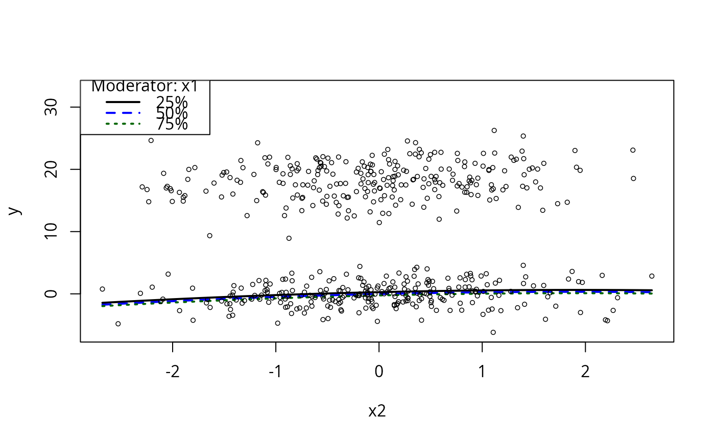
plotCurves(m1, plotx = "x2", modx = "x1")
## ## Verify that plot by comparing against a manually contructed alternative
## par(mfrow=c(1,2))
## plotCurves(m1, plotx = "x1", modx = "xcat1")
## newdat <- with(dat, expand.grid(x1 = plotSeq(x1, 30), xcat1 = levels(xcat1)))
## newdat$x2 <- with(dat, mean(x2, na.rm = TRUE))
## newdat$m1p <- predict(m1, newdata = newdat)
## plot( y ~ x1, data = dat, type = "n", ylim = magRange(dat$y, c(1, 1.2)))
## points( y ~ x1, data = dat, col = dat$xcat1, cex = 0.4, lwd = 0.5)
## by(newdat, newdat$xcat1, function(dd) {lines(dd$x1, dd$m1p)})
## legend("topleft", legend=levels(dat$xcat1), col = as.numeric(dat$xcat1), lty = 1)
## par(mfrow = c(1,1))
## ##Close enough!
plotCurves(m1, plotx = "x2", modx = "x1")
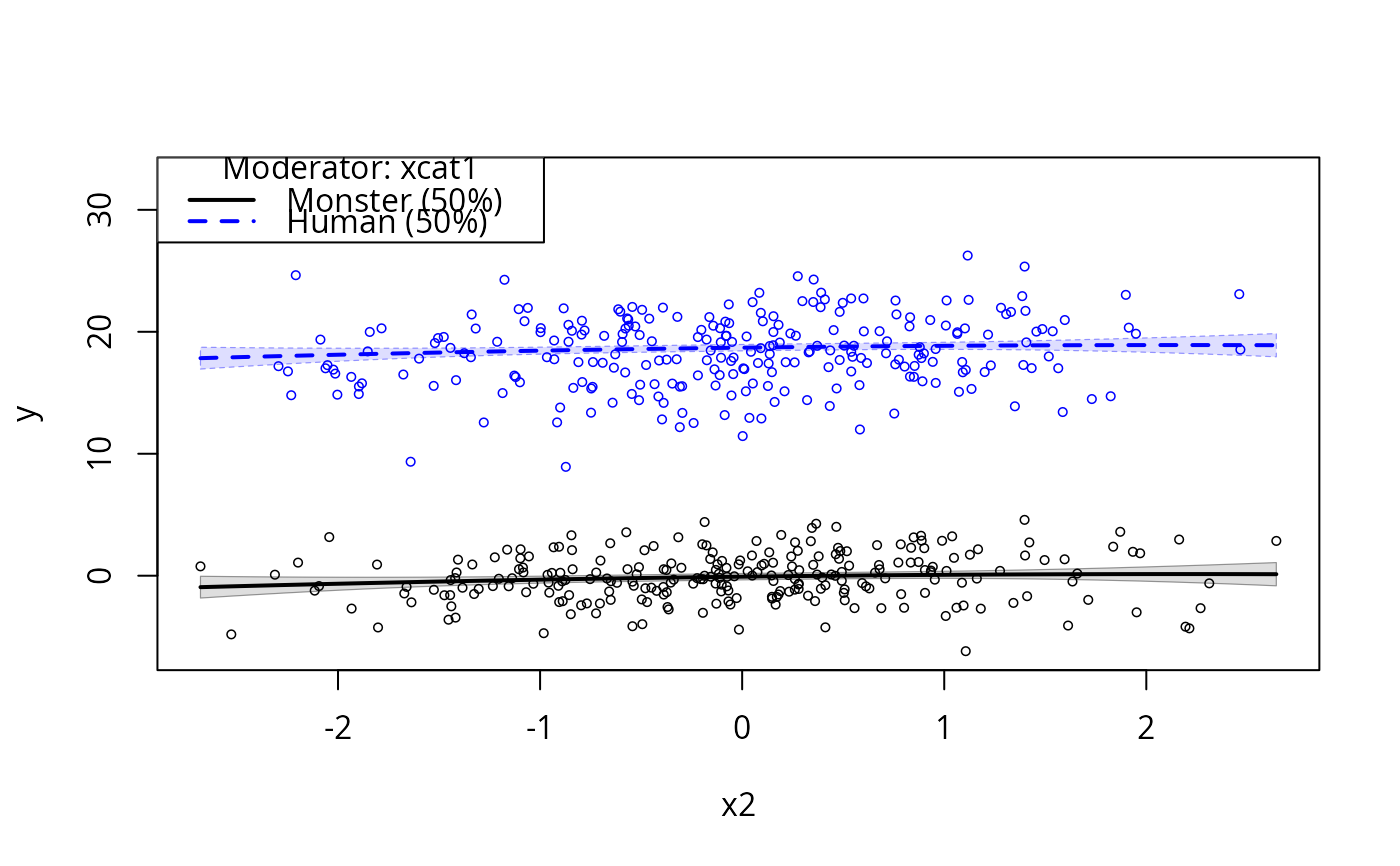
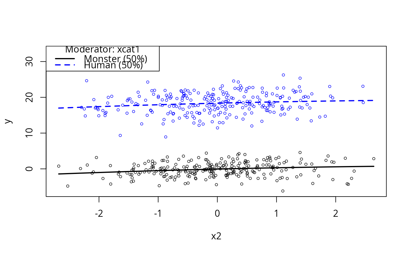
 plotCurves(m1, plotx = "x2", modx = "xcat1")
 plotCurves(m1, plotx = "x2", modx = "xcat1", interval = "conf")
 m2 <- lm(y ~ log(x1)*xcat1 + xcat1*(x2 + I(x2^2)), data = dat)
summary(m2)
#>
#> Call:
#> lm(formula = y ~ log(x1) * xcat1 + xcat1 * (x2 + I(x2^2)), data = dat)
#>
#> Residuals:
#> Min 1Q Median 3Q Max
#> -6.4211 -1.1936 -0.0554 1.2288 4.9131
#>
#> Coefficients:
#> Estimate Std. Error t value Pr(>|t|)
#> (Intercept) 3.00314 0.92528 3.246 0.00125 **
#> log(x1) -1.87872 0.57457 -3.270 0.00115 **
#> xcat1Human -3.16751 1.32882 -2.384 0.01752 *
#> x2 0.37497 0.12205 3.072 0.00224 **
#> I(x2^2) -0.09868 0.08742 -1.129 0.25951
#> log(x1):xcat1Human 13.56145 0.82871 16.365 < 2e-16 ***
#> xcat1Human:x2 -0.34460 0.17349 -1.986 0.04756 *
#> xcat1Human:I(x2^2) 0.09449 0.12889 0.733 0.46383
#> ---
#> Signif. codes: 0 ‘***’ 0.001 ‘**’ 0.01 ‘*’ 0.05 ‘.’ 0.1 ‘ ’ 1
#>
#> Residual standard error: 1.851 on 492 degrees of freedom
#> Multiple R-squared: 0.9629, Adjusted R-squared: 0.9624
#> F-statistic: 1827 on 7 and 492 DF, p-value: < 2.2e-16
#>
plotCurves(m2, plotx = "x2", modx = "xcat1")
m2 <- lm(y ~ log(x1)*xcat1 + xcat1*(x2 + I(x2^2)), data = dat)
summary(m2)
#>
#> Call:
#> lm(formula = y ~ log(x1) * xcat1 + xcat1 * (x2 + I(x2^2)), data = dat)
#>
#> Residuals:
#> Min 1Q Median 3Q Max
#> -6.4211 -1.1936 -0.0554 1.2288 4.9131
#>
#> Coefficients:
#> Estimate Std. Error t value Pr(>|t|)
#> (Intercept) 3.00314 0.92528 3.246 0.00125 **
#> log(x1) -1.87872 0.57457 -3.270 0.00115 **
#> xcat1Human -3.16751 1.32882 -2.384 0.01752 *
#> x2 0.37497 0.12205 3.072 0.00224 **
#> I(x2^2) -0.09868 0.08742 -1.129 0.25951
#> log(x1):xcat1Human 13.56145 0.82871 16.365 < 2e-16 ***
#> xcat1Human:x2 -0.34460 0.17349 -1.986 0.04756 *
#> xcat1Human:I(x2^2) 0.09449 0.12889 0.733 0.46383
#> ---
#> Signif. codes: 0 ‘***’ 0.001 ‘**’ 0.01 ‘*’ 0.05 ‘.’ 0.1 ‘ ’ 1
#>
#> Residual standard error: 1.851 on 492 degrees of freedom
#> Multiple R-squared: 0.9629, Adjusted R-squared: 0.9624
#> F-statistic: 1827 on 7 and 492 DF, p-value: < 2.2e-16
#>
plotCurves(m2, plotx = "x2", modx = "xcat1")
 plotCurves(m2, plotx ="x2", modx = "x1")
 m3a <- lm(y ~ poly(x2, 2) + xcat1, data = dat)
plotCurves(m3a, plotx = "x2")
m3a <- lm(y ~ poly(x2, 2) + xcat1, data = dat)
plotCurves(m3a, plotx = "x2")
 plotCurves(m3a, plotx = "x2", modx = "xcat1")
 #OK
m4 <- lm(log(y+10) ~ poly(x2, 2)*xcat1 + x1, data = dat)
summary(m4)
#>
#> Call:
#> lm(formula = log(y + 10) ~ poly(x2, 2) * xcat1 + x1, data = dat)
#>
#> Residuals:
#> Min 1Q Median 3Q Max
#> -0.95025 -0.07313 0.00750 0.09019 0.43193
#>
#> Coefficients:
#> Estimate Std. Error t value Pr(>|t|)
#> (Intercept) 2.166865 0.040326 53.734 <2e-16 ***
#> poly(x2, 2)1 0.484173 0.239110 2.025 0.0434 *
#> poly(x2, 2)2 -0.540927 0.226887 -2.384 0.0175 *
#> xcat1Human 1.069861 0.014881 71.895 <2e-16 ***
#> x1 0.020319 0.007702 2.638 0.0086 **
#> poly(x2, 2)1:xcat1Human -0.152951 0.333419 -0.459 0.6466
#> poly(x2, 2)2:xcat1Human 0.587847 0.334495 1.757 0.0795 .
#> ---
#> Signif. codes: 0 ‘***’ 0.001 ‘**’ 0.01 ‘*’ 0.05 ‘.’ 0.1 ‘ ’ 1
#>
#> Residual standard error: 0.1662 on 493 degrees of freedom
#> Multiple R-squared: 0.9131, Adjusted R-squared: 0.9121
#> F-statistic: 863.5 on 6 and 493 DF, p-value: < 2.2e-16
#>
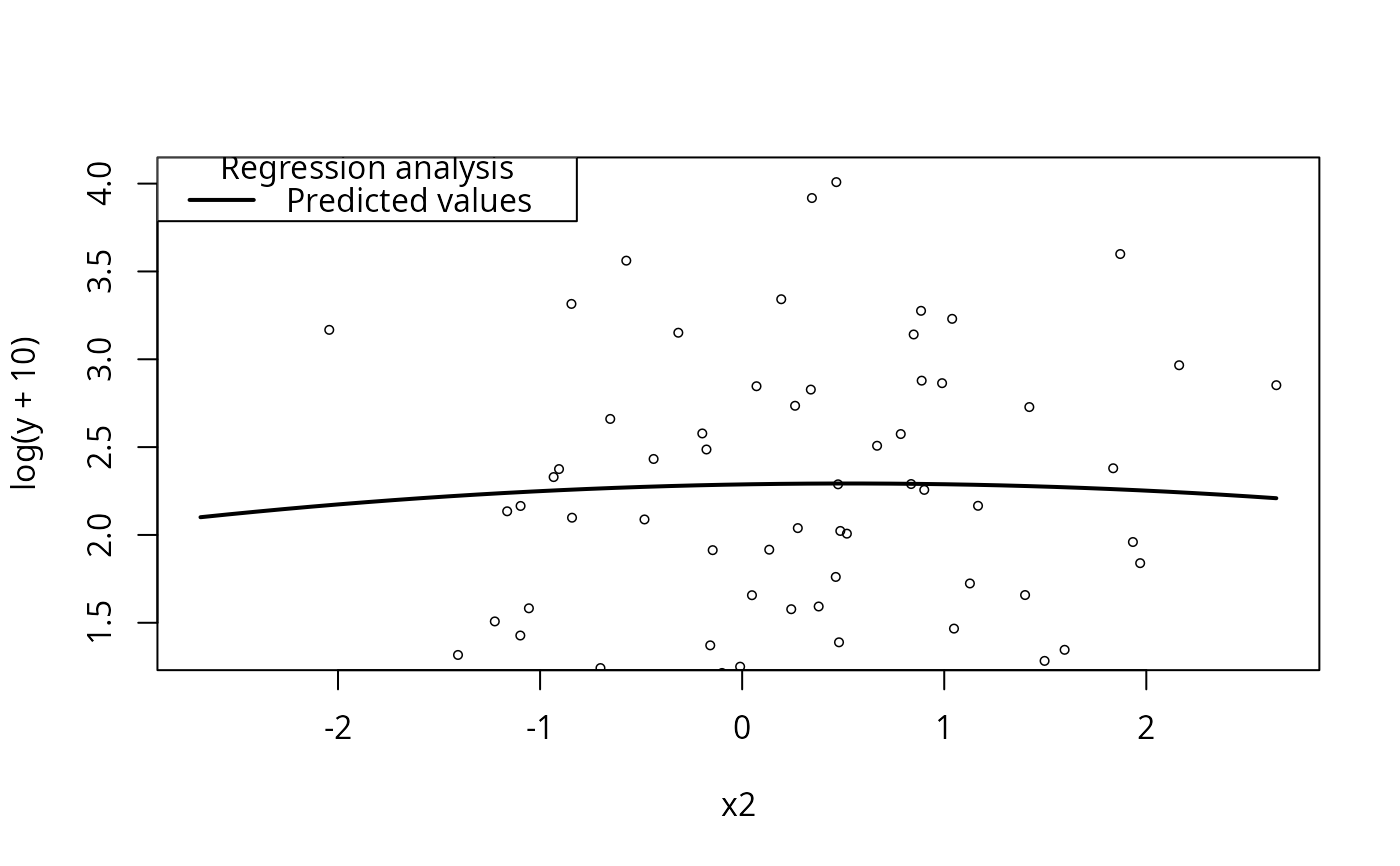
plotCurves(m4, plotx = "x2")
#OK
m4 <- lm(log(y+10) ~ poly(x2, 2)*xcat1 + x1, data = dat)
summary(m4)
#>
#> Call:
#> lm(formula = log(y + 10) ~ poly(x2, 2) * xcat1 + x1, data = dat)
#>
#> Residuals:
#> Min 1Q Median 3Q Max
#> -0.95025 -0.07313 0.00750 0.09019 0.43193
#>
#> Coefficients:
#> Estimate Std. Error t value Pr(>|t|)
#> (Intercept) 2.166865 0.040326 53.734 <2e-16 ***
#> poly(x2, 2)1 0.484173 0.239110 2.025 0.0434 *
#> poly(x2, 2)2 -0.540927 0.226887 -2.384 0.0175 *
#> xcat1Human 1.069861 0.014881 71.895 <2e-16 ***
#> x1 0.020319 0.007702 2.638 0.0086 **
#> poly(x2, 2)1:xcat1Human -0.152951 0.333419 -0.459 0.6466
#> poly(x2, 2)2:xcat1Human 0.587847 0.334495 1.757 0.0795 .
#> ---
#> Signif. codes: 0 ‘***’ 0.001 ‘**’ 0.01 ‘*’ 0.05 ‘.’ 0.1 ‘ ’ 1
#>
#> Residual standard error: 0.1662 on 493 degrees of freedom
#> Multiple R-squared: 0.9131, Adjusted R-squared: 0.9121
#> F-statistic: 863.5 on 6 and 493 DF, p-value: < 2.2e-16
#>
plotCurves(m4, plotx = "x2")
 plotCurves(m4, plotx ="x2", modx = "xcat1")
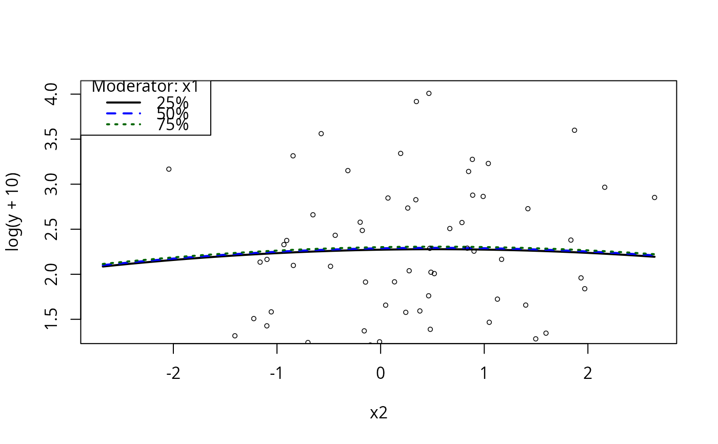
 plotCurves(m4, plotx = "x2", modx = "x1")
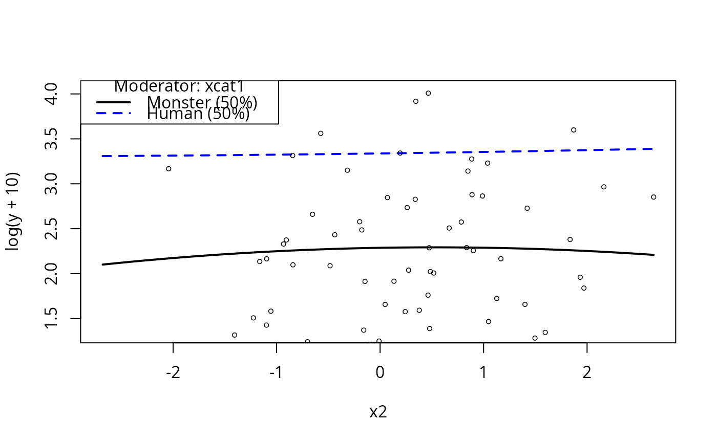
 plotCurves(m4, plotx = "x2", modx = "xcat1")
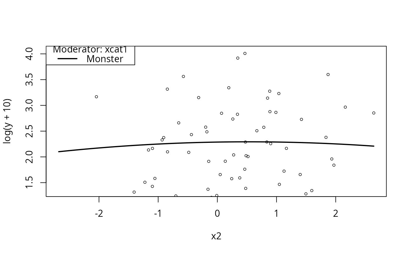
 plotCurves(m4, plotx = "x2", modx = "xcat1", modxVals = c("Monster"))
 ##ordinary interaction
m5 <- lm(y2 ~ x1*x2 + x3 +x4, data = dat)
summary(m5)
#>
#> Call:
#> lm(formula = y2 ~ x1 * x2 + x3 + x4, data = dat)
#>
#> Residuals:
#> Min 1Q Median 3Q Max
#> -3.3410 -0.6731 -0.0192 0.6530 2.4076
#>
#> Coefficients:
#> Estimate Std. Error t value Pr(>|t|)
#> (Intercept) -0.14712 0.23815 -0.618 0.53701
#> x1 0.14875 0.04647 3.201 0.00146 **
#> x2 0.19880 0.23772 0.836 0.40340
#> x3 0.38256 0.04403 8.688 < 2e-16 ***
#> x4 -0.03070 0.04479 -0.685 0.49343
#> x1:x2 0.21975 0.04578 4.800 2.11e-06 ***
#> ---
#> Signif. codes: 0 ‘***’ 0.001 ‘**’ 0.01 ‘*’ 0.05 ‘.’ 0.1 ‘ ’ 1
#>
#> Residual standard error: 0.966 on 494 degrees of freedom
#> Multiple R-squared: 0.7027, Adjusted R-squared: 0.6996
#> F-statistic: 233.5 on 5 and 494 DF, p-value: < 2.2e-16
#>
plotCurves(m5, plotx = "x1", modx = "x2")
##ordinary interaction
m5 <- lm(y2 ~ x1*x2 + x3 +x4, data = dat)
summary(m5)
#>
#> Call:
#> lm(formula = y2 ~ x1 * x2 + x3 + x4, data = dat)
#>
#> Residuals:
#> Min 1Q Median 3Q Max
#> -3.3410 -0.6731 -0.0192 0.6530 2.4076
#>
#> Coefficients:
#> Estimate Std. Error t value Pr(>|t|)
#> (Intercept) -0.14712 0.23815 -0.618 0.53701
#> x1 0.14875 0.04647 3.201 0.00146 **
#> x2 0.19880 0.23772 0.836 0.40340
#> x3 0.38256 0.04403 8.688 < 2e-16 ***
#> x4 -0.03070 0.04479 -0.685 0.49343
#> x1:x2 0.21975 0.04578 4.800 2.11e-06 ***
#> ---
#> Signif. codes: 0 ‘***’ 0.001 ‘**’ 0.01 ‘*’ 0.05 ‘.’ 0.1 ‘ ’ 1
#>
#> Residual standard error: 0.966 on 494 degrees of freedom
#> Multiple R-squared: 0.7027, Adjusted R-squared: 0.6996
#> F-statistic: 233.5 on 5 and 494 DF, p-value: < 2.2e-16
#>
plotCurves(m5, plotx = "x1", modx = "x2")
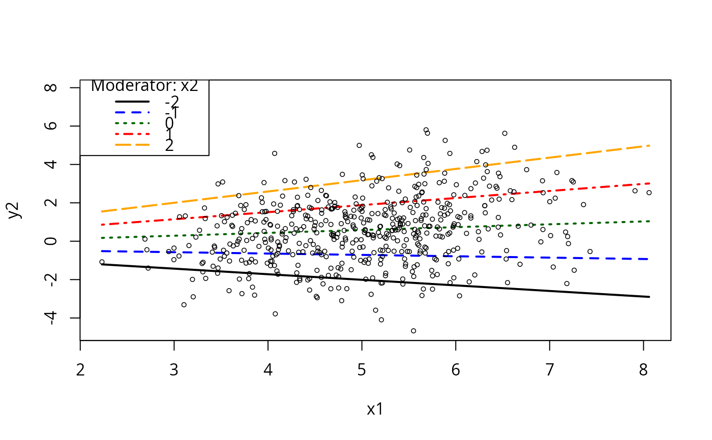
 plotCurves(m5, plotx = "x1", modx = "x2", modxVals = c( -2, -1, 0, 1, 2))
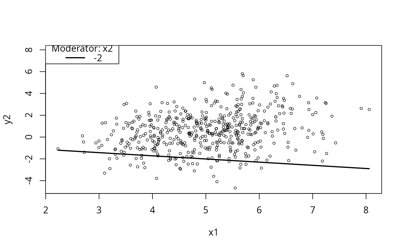
 plotCurves(m5, plotx = "x1", modx = "x2", modxVals = c(-2))
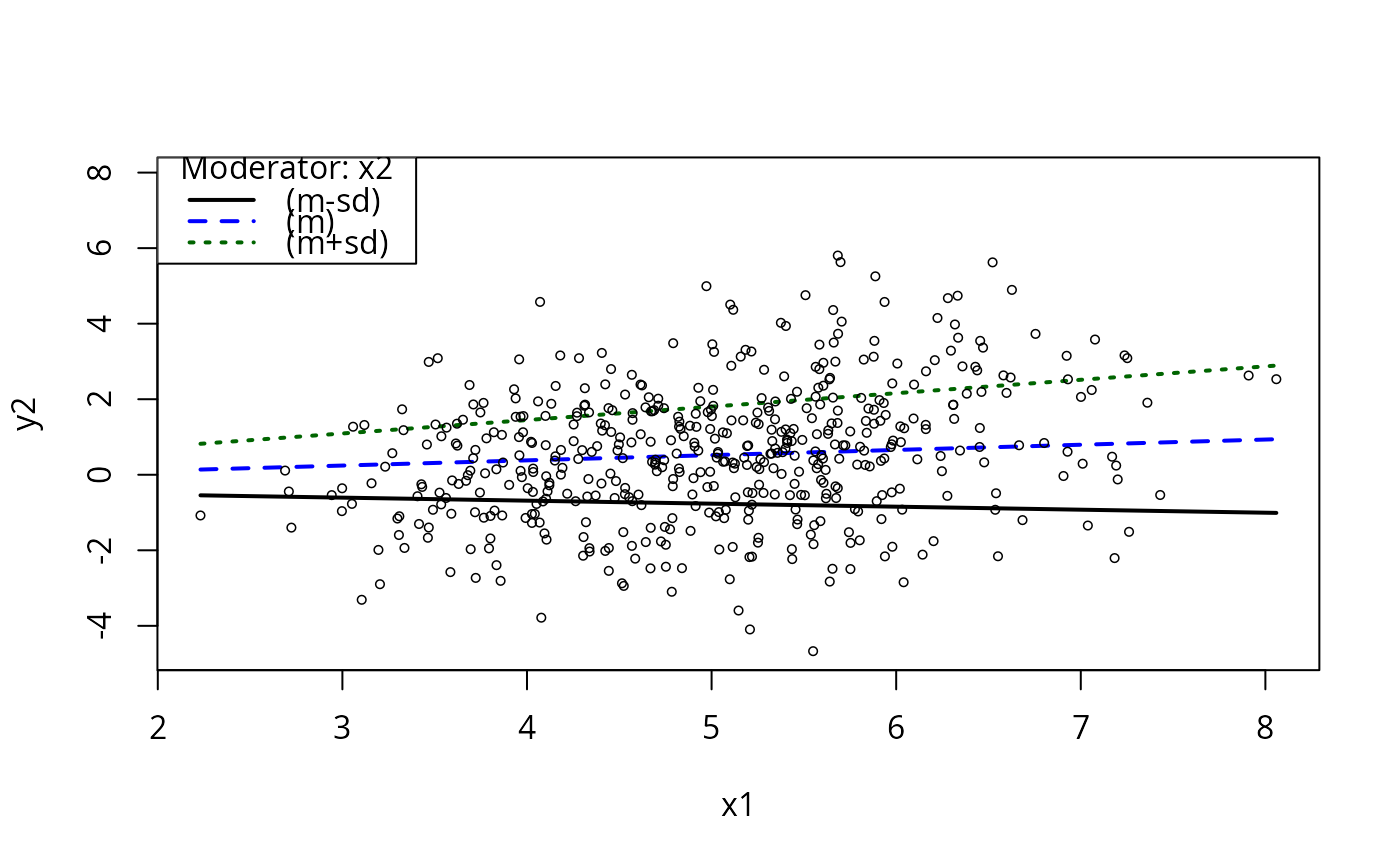
 plotCurves(m5, plotx = "x1", modx = "x2", modxVals = "std.dev.")
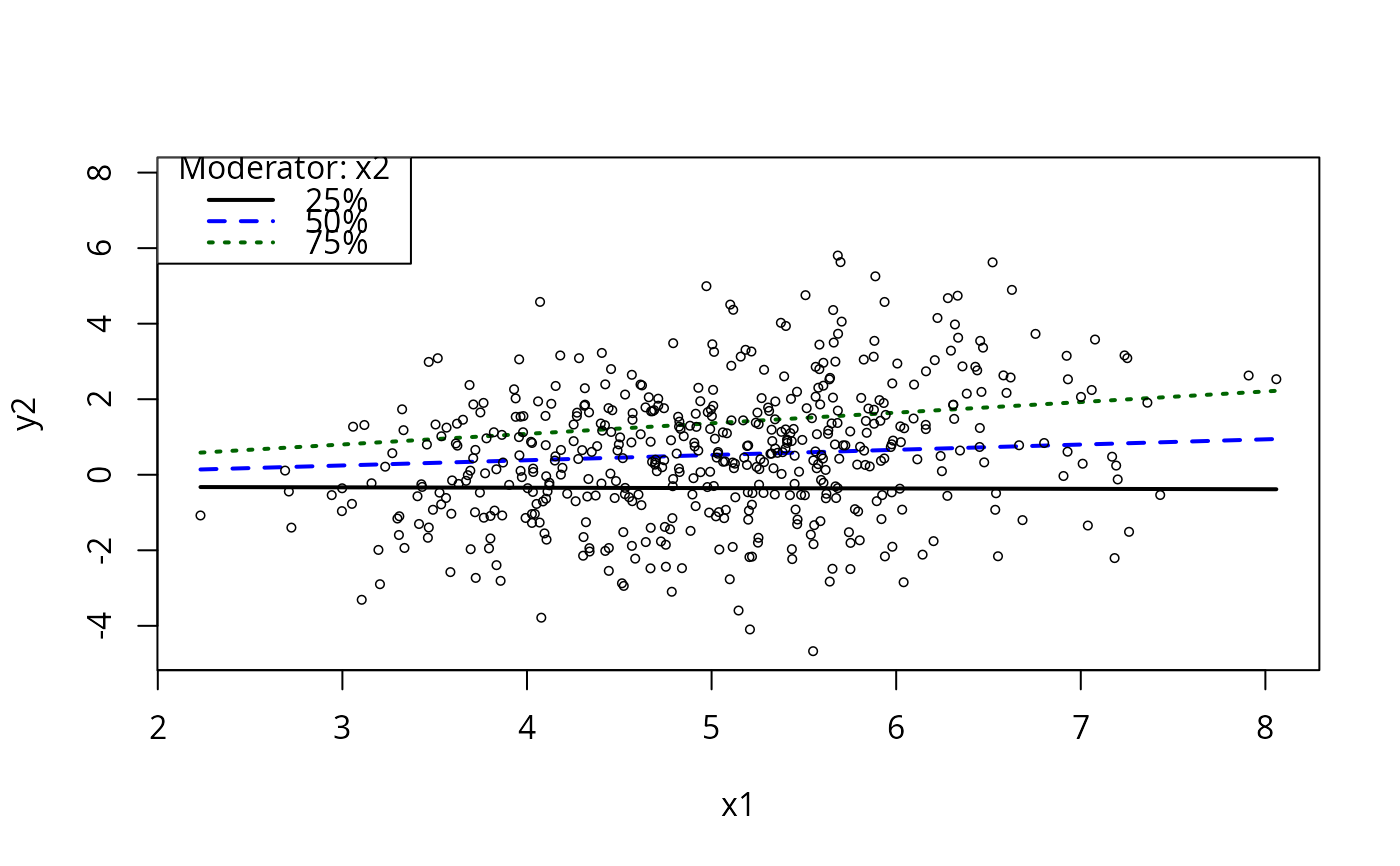
 plotCurves(m5, plotx = "x1", modx = "x2", modxVals = "quantile")
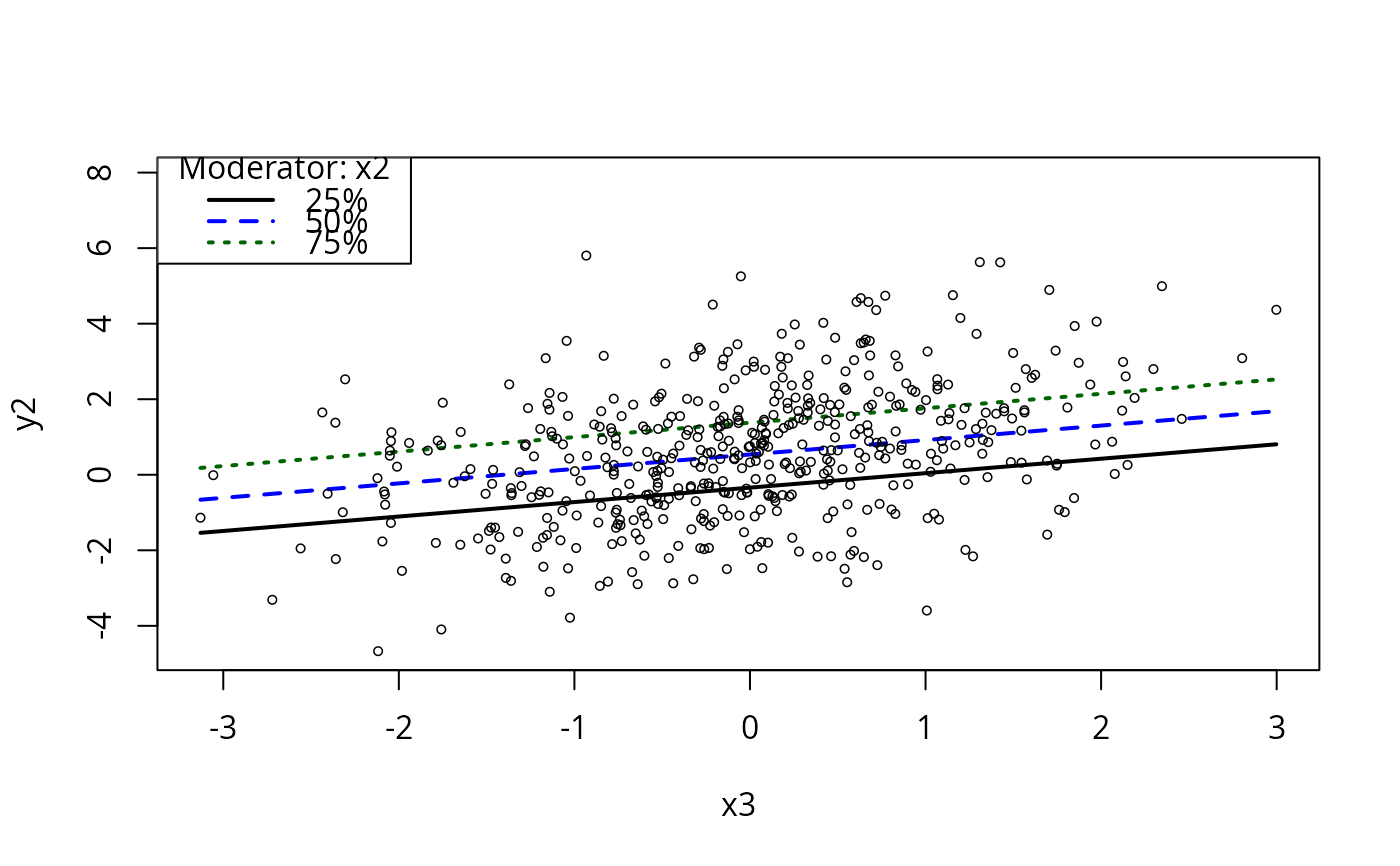
 plotCurves(m5, plotx = "x3", modx = "x2")
 if(require(carData)){
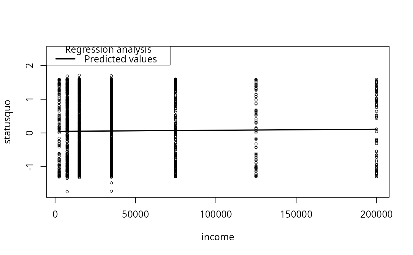
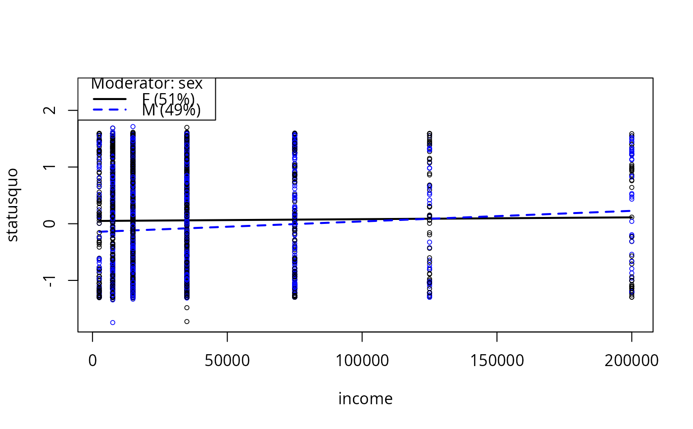
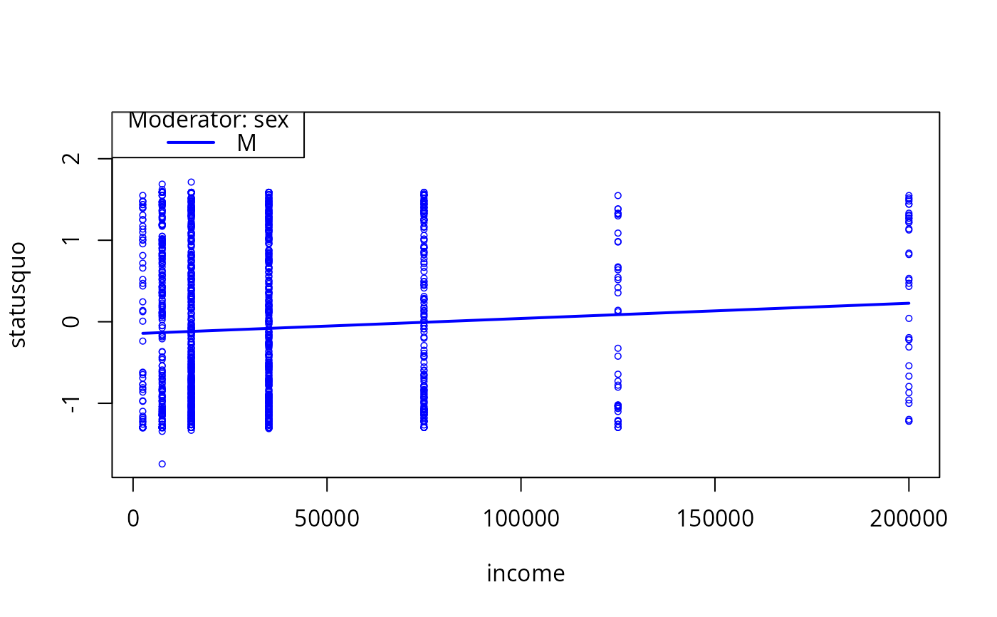
mc1 <- lm(statusquo ~ income * sex, data = Chile)
summary(mc1)
plotCurves(mc1, plotx = "income")
plotCurves(mc1, modx = "sex", plotx = "income")
plotCurves(mc1, modx = "sex", plotx = "income", modxVals = "M")
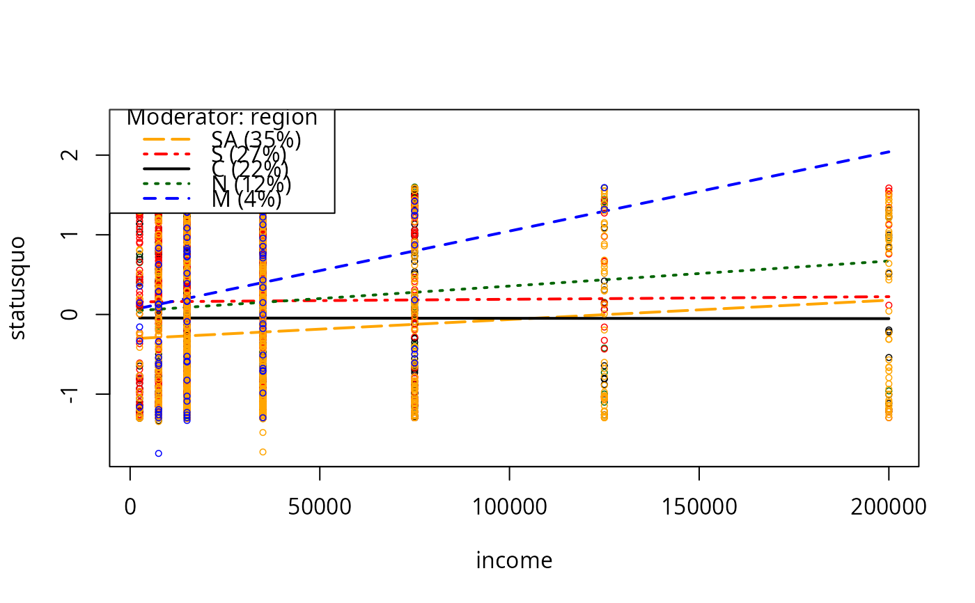
mc2 <- lm(statusquo ~ region * income, data = Chile)
summary(mc2)
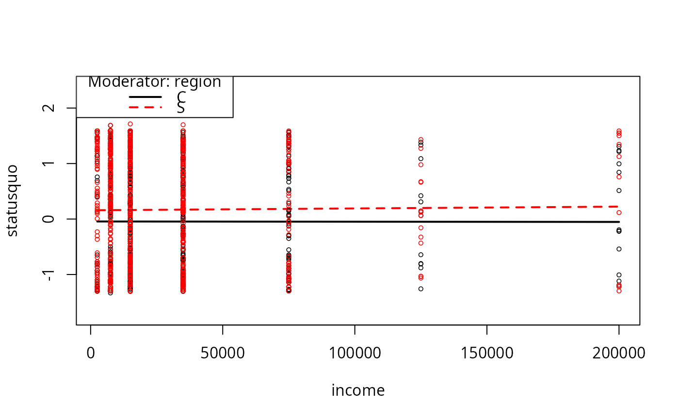
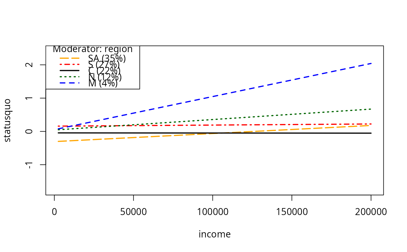
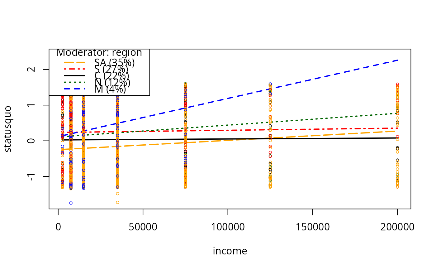
plotCurves(mc2, modx = "region", plotx = "income")
plotCurves(mc2, modx = "region", plotx = "income",
modxVals = levels(Chile$region)[c(1,4)])
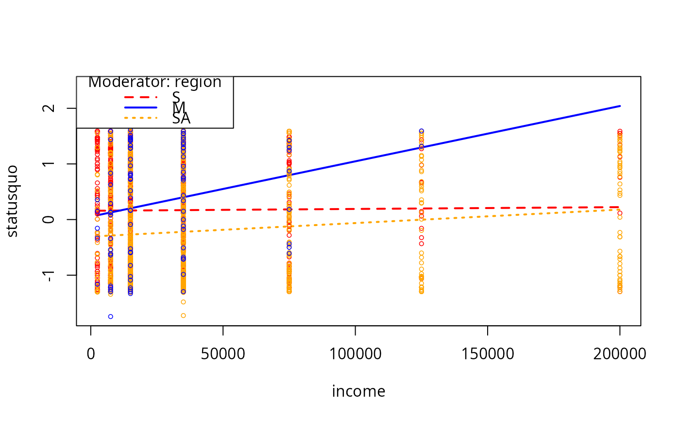
plotCurves(mc2, modx = "region", plotx = "income", modxVals = c("S","M","SA"))
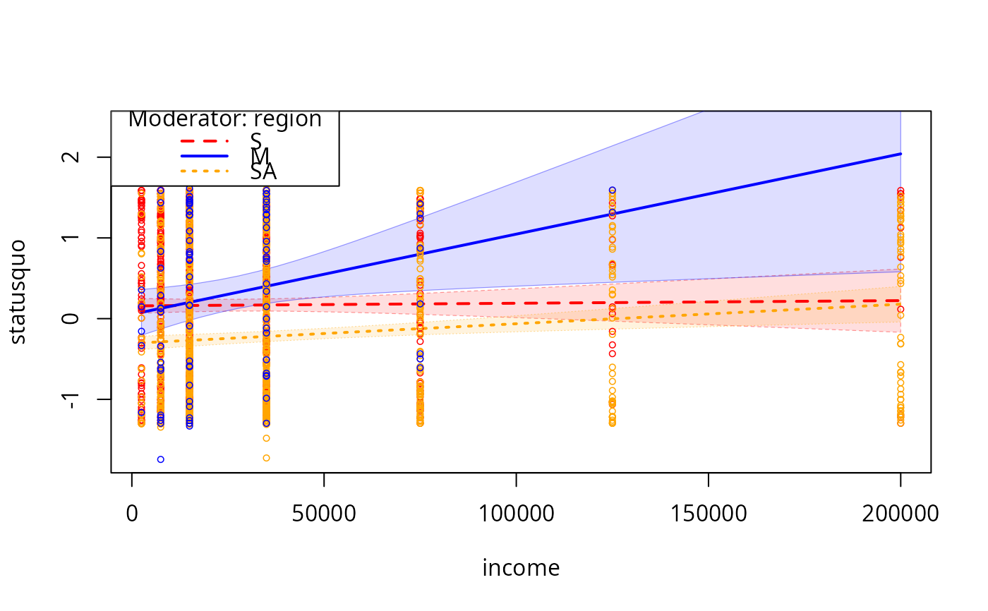
plotCurves(mc2, modx = "region", plotx = "income", modxVals = c("S","M","SA"),
interval = "conf")
plotCurves(mc2, modx = "region", plotx = "income", plotPoints = FALSE)
mc3 <- lm(statusquo ~ region * income + sex + age, data = Chile)
summary(mc3)
plotCurves(mc3, modx = "region", plotx = "income")
mc4 <- lm(statusquo ~ income * (age + I(age^2)) + education + sex + age, data = Chile)
summary(mc4)
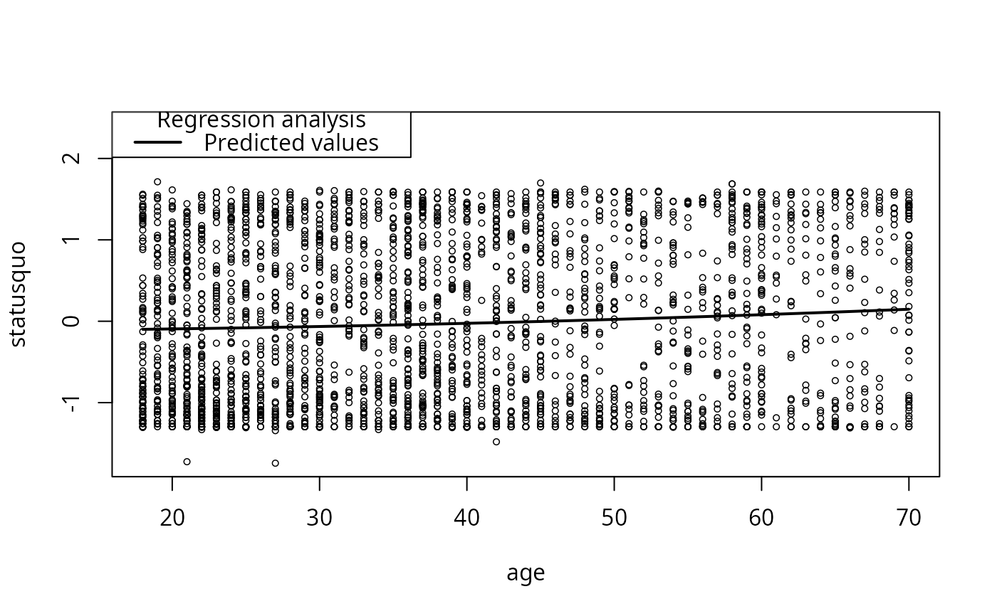
plotCurves(mc4, plotx = "age")
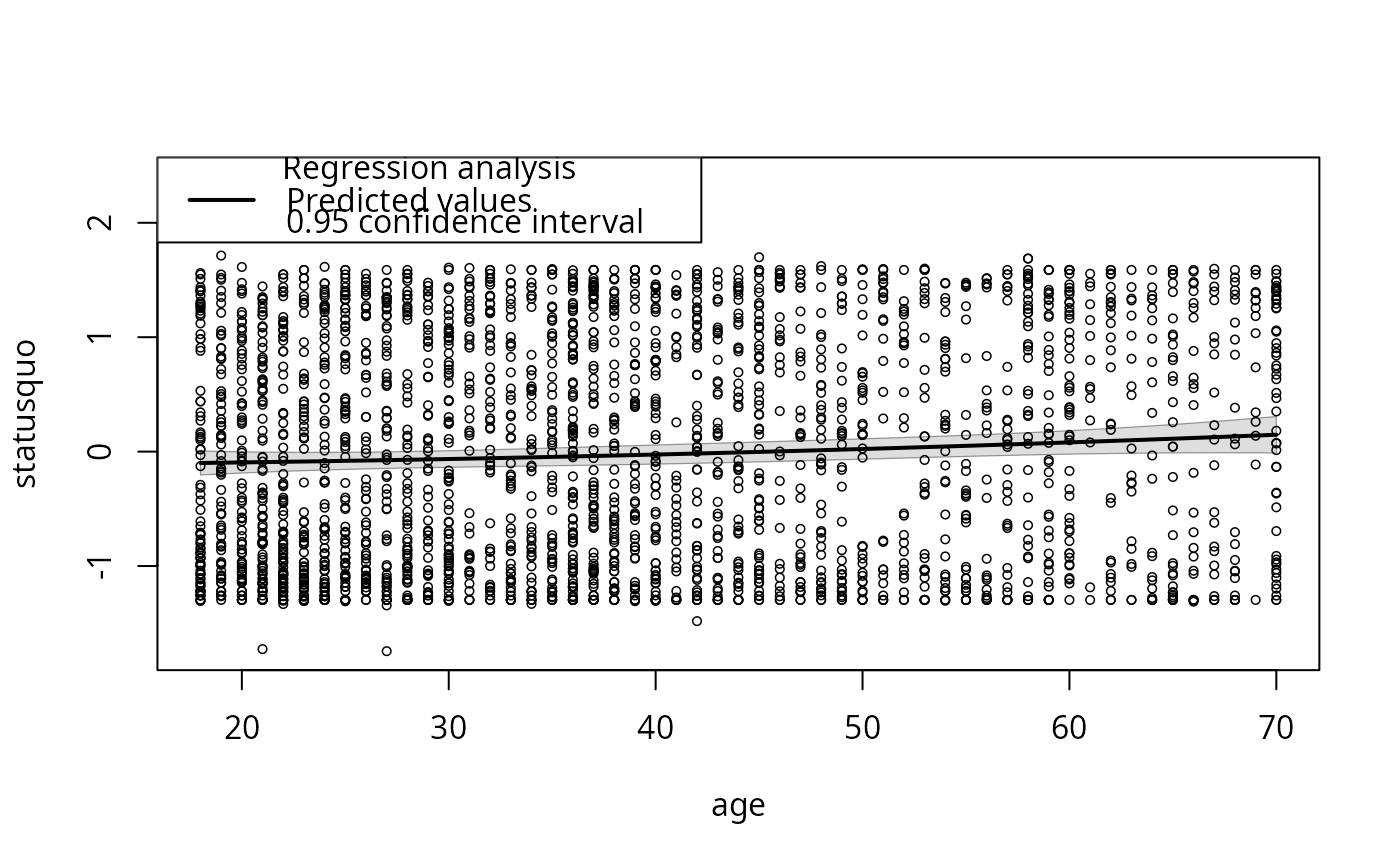
plotCurves(mc4, plotx = "age", interval = "conf")
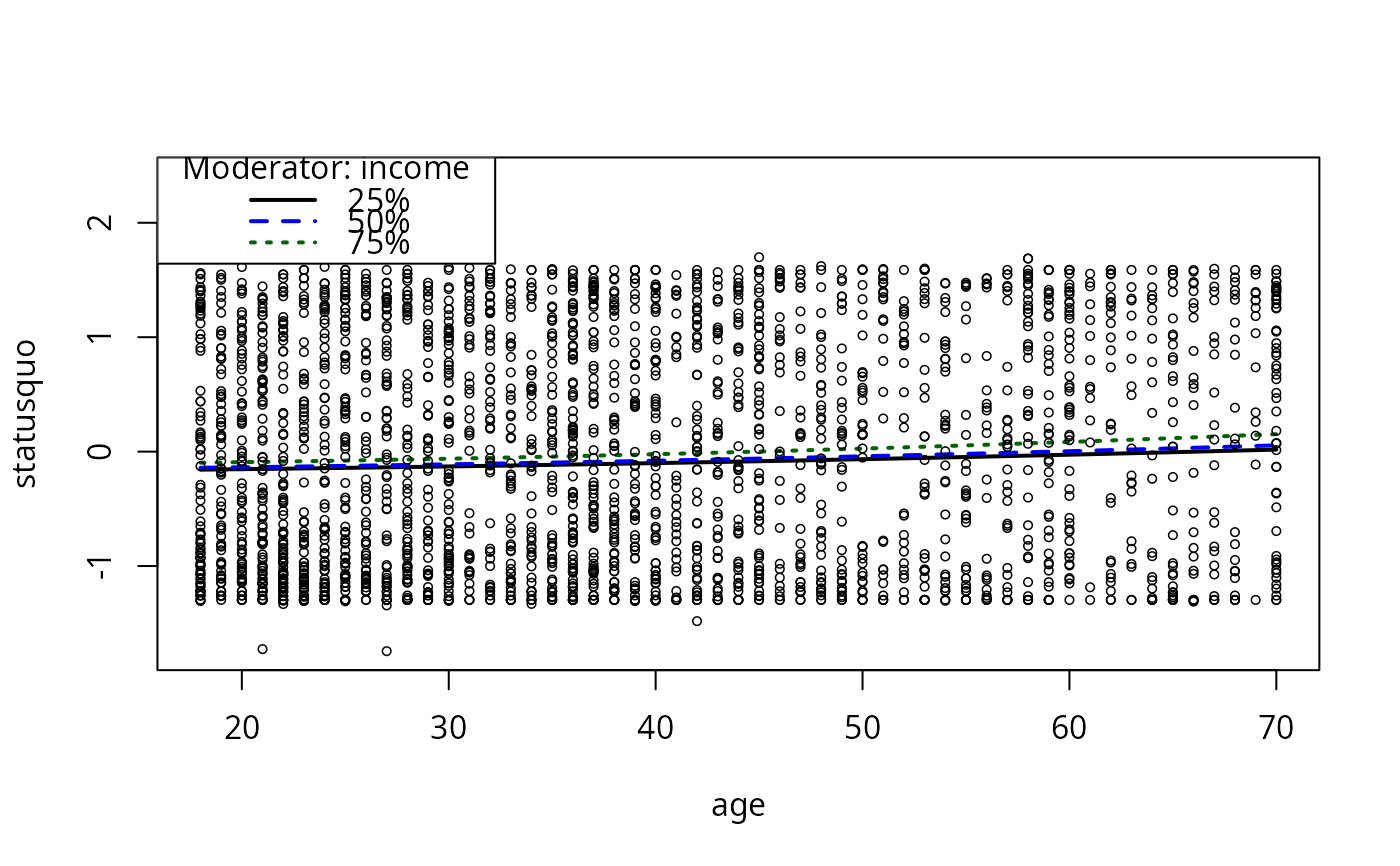
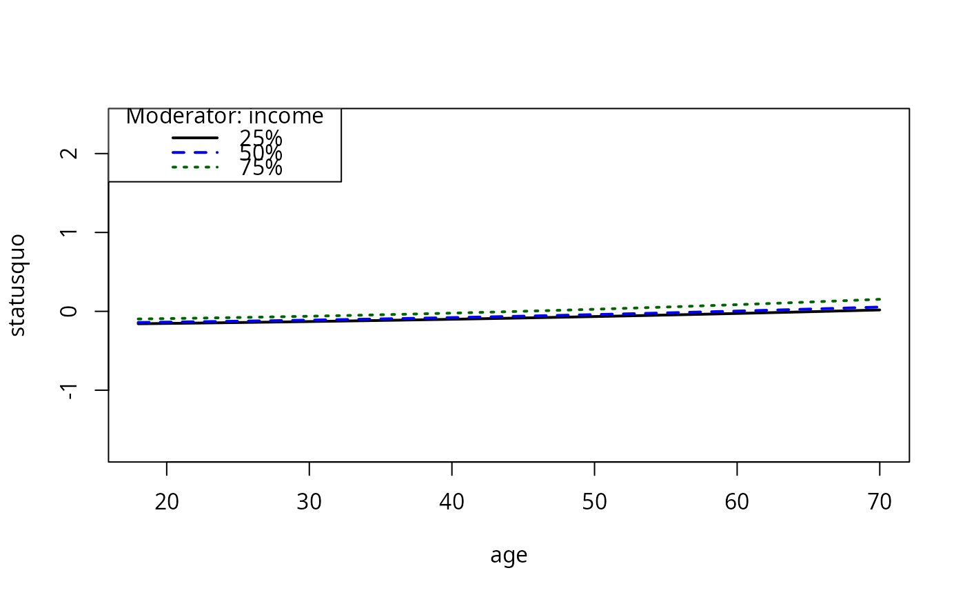
plotCurves(mc4, plotx = "age", modx = "income")
plotCurves(mc4, plotx = "age", modx = "income", plotPoints = FALSE)
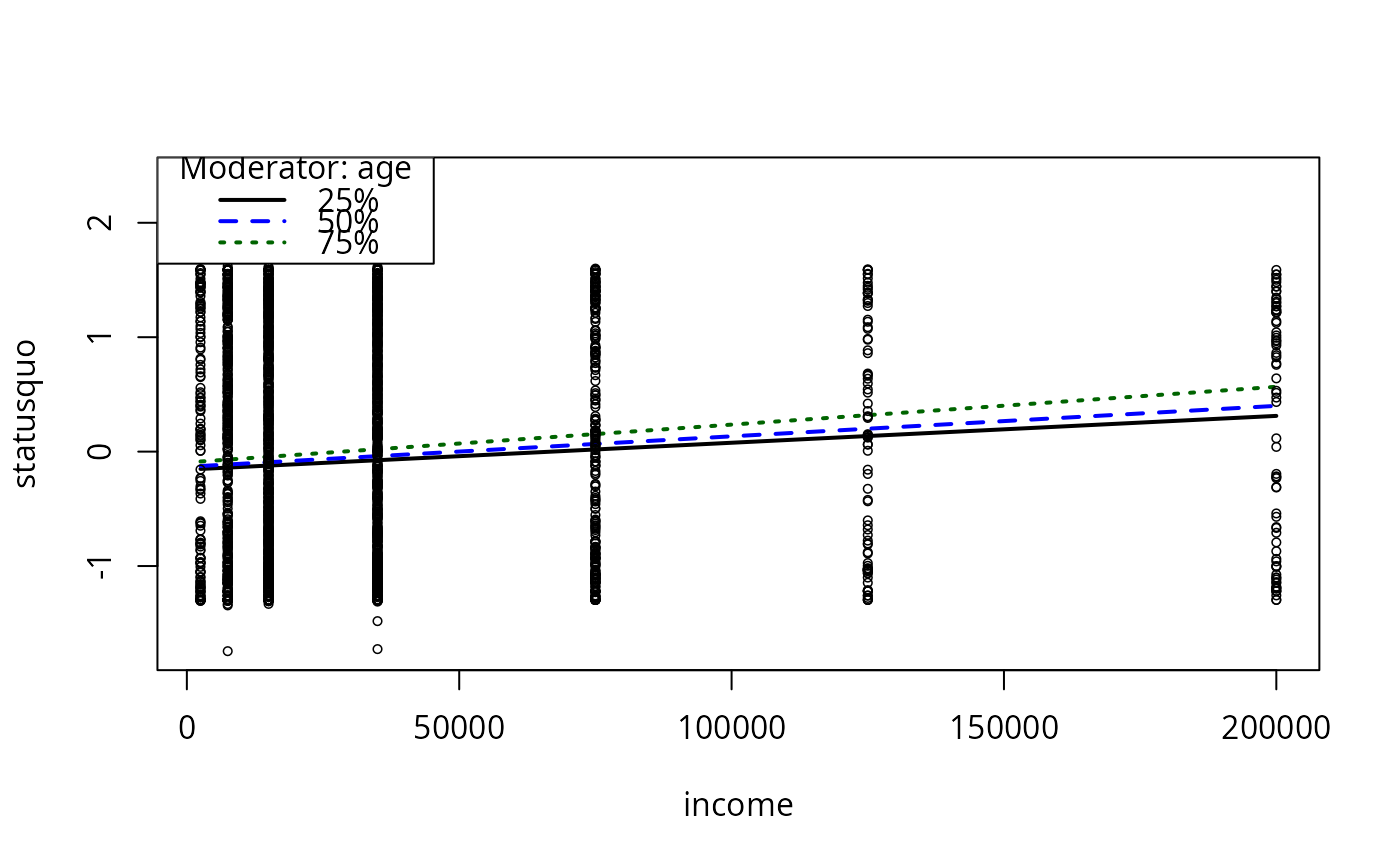
plotCurves(mc4, plotx = "income", modx = "age")
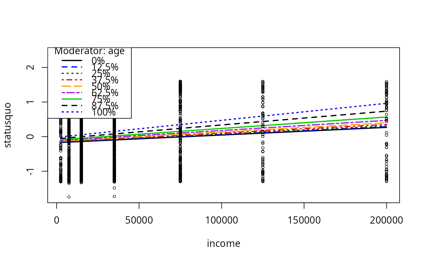
plotCurves(mc4, plotx = "income", modx = "age", n = 8)
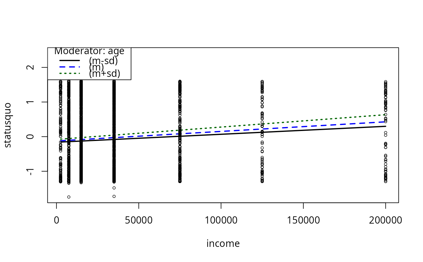
plotCurves(mc4, plotx = "income", modx = "age", modxVals = "std.dev.")
plotCurves(mc4, modx = "income", plotx = "age", plotPoints = FALSE)
}
#> Loading required package: carData
if(require(carData)){
mc1 <- lm(statusquo ~ income * sex, data = Chile)
summary(mc1)
plotCurves(mc1, plotx = "income")
plotCurves(mc1, modx = "sex", plotx = "income")
plotCurves(mc1, modx = "sex", plotx = "income", modxVals = "M")
mc2 <- lm(statusquo ~ region * income, data = Chile)
summary(mc2)
plotCurves(mc2, modx = "region", plotx = "income")
plotCurves(mc2, modx = "region", plotx = "income",
modxVals = levels(Chile$region)[c(1,4)])
plotCurves(mc2, modx = "region", plotx = "income", modxVals = c("S","M","SA"))
plotCurves(mc2, modx = "region", plotx = "income", modxVals = c("S","M","SA"),
interval = "conf")
plotCurves(mc2, modx = "region", plotx = "income", plotPoints = FALSE)
mc3 <- lm(statusquo ~ region * income + sex + age, data = Chile)
summary(mc3)
plotCurves(mc3, modx = "region", plotx = "income")
mc4 <- lm(statusquo ~ income * (age + I(age^2)) + education + sex + age, data = Chile)
summary(mc4)
plotCurves(mc4, plotx = "age")
plotCurves(mc4, plotx = "age", interval = "conf")
plotCurves(mc4, plotx = "age", modx = "income")
plotCurves(mc4, plotx = "age", modx = "income", plotPoints = FALSE)
plotCurves(mc4, plotx = "income", modx = "age")
plotCurves(mc4, plotx = "income", modx = "age", n = 8)
plotCurves(mc4, plotx = "income", modx = "age", modxVals = "std.dev.")
plotCurves(mc4, modx = "income", plotx = "age", plotPoints = FALSE)
}
#> Loading required package: carData