Generates a data frame for regression analysis.
genCorrelatedData2.RdUnlike genCorrelatedData, this new-and-improved
function can generate a data frame with as many predictors
as the user requests along with an arbitrarily complicated
regression formula. The result will be a data frame with
columns named (y, x1, x2, ..., xp).
Arguments
- N
Number of cases desired
- means
P-vector of means for X. Implicitly sets the dimension of the predictor matrix as N x P.
- sds
Values for standard deviations for columns of X. If less than P values are supplied, they will be recycled.
- rho
Correlation coefficient for X. Several input formats are allowed (see
lazyCor). This can be a single number (common correlation among all variables), a full matrix of correlations among all variables, or a vector that is interpreted as the strictly lower triangle (a vech).- stde
standard deviation of the error term in the data generating equation
- beta
beta vector of coefficients for intercept, slopes, and interaction terma. The first P+1 values are the intercept and slope coefficients for the predictors. Additional elements in beta are interpreted as coefficients for nonlinear and interaction coefficients. I have decided to treat these as a column (vech) that fills into a lower triangular matrix. It is easy to see what's going on if you run the examples. There is also explanation in Details.
- intercept
Default FALSE. Should the predictors include an intercept?
- verbose
TRUE or FALSE. Should information about the data generation be reported to the terminal?
Details
Arguments supplied must have enough information so that an
N x P matrix of predictors can be constructed.
The matrix X is drawn from a multivariate normal
distribution, the expected value vector (mu vector) is given by
the means and the var/covar matrix (Sigma) is
built from user supplied standard deviations sds
and the correlations between the columns of X, given by rho.
The user can also set the standard deviation
of the error term (stde) and the coefficients
of the regression equation (beta).
If called with no arguments, this creates a data frame with X ~ MVN(mu = c(50,50,50), Sigma = diag(c(10,10,10))). y = X is N(m = 0, sd = 200). All of these details can be changed by altering the arguments.
The y (output) variable is created according to the
equation
$$
y = b1 + b2 * x1 + ...+ bk * xk + b[k+1] * x1 * ...interactions.. + e$$
For shorthand, I write b1 for beta[1], b2 for beta[2], and so forth.
The first P+1 arguments in the argument beta are the coefficients
for the intercept and the columns of the X matrix. Any additional
elements in beta are the coefficients for nonlinear and interaction terms.
Those additional values in the beta vector are completely
optional. Without them, the true model is a linear
regression. However, one can incorporate the effect of squared terms
(conceptualize that as x1 * x1, for example) or interactions
(x1 * x2) easily. This is easier to illustrate than describe.
Suppose there are 4 columns in X. Then a beta
vector like beta = c(0, 1, 2, 3, 4, 5, 6, 7, 8) would amount to
asking for
$$
y = 0 + 1 x1 + 2 x2 + 3 x3 + 4 x4 + 5 x1^2 + 6 x1 x2 + 7 x1 x3 + 8 x1 x4 + error
$$
If beta supplies more coefficients, they are interpeted as additional
interactions.
When there are a many predictors and the beta vector is long, this
can become confusing. I think of this as a vech for the lower
triangle of a coefficient matrix. In the example with 4
predictors, beta[1:5] are used for the intercepts and slopes. The
rest of the beta elements lay in like so:
X1 X2 X3 X4
X1 b6 . .
X2 b7 b10 .
X3 b8 b11 b13
X4 b9 b12 b14 b15
If the user only supplies b6 and b7, the rest are assumed to be 0.
To make this clear, the formula used to calculate y is printed to the console when genCorrelatedData2 is called.
Examples
## 1000 observations of uncorrelated X with no interactions
set.seed(234234)
dat <- genCorrelatedData2(N = 10, rho = 0.0, beta = c(1, 2, 1, 1),
means = c(0,0,0), sds = c(1,1,1), stde = 0)
#> [1] "The equation that was calculated was"
#> y = 1 + 2*x1 + 1*x2 + 1*x3
#> + 0*x1*x1 + 0*x2*x1 + 0*x3*x1
#> + 0*x1*x2 + 0*x2*x2 + 0*x3*x2
#> + 0*x1*x3 + 0*x2*x3 + 0*x3*x3
#> + N(0,0) random error
summarize(dat)
#> Numeric variables
#> y x1 x2 x3
#> min -1.225 -1.410 -1.454 -1.968
#> med 0.313 -0.070 -0.275 -0.014
#> max 2.871 1.001 1.864 0.878
#> mean 0.547 -0.057 -0.065 -0.273
#> sd 1.294 0.797 1.092 0.830
#> skewness 0.322 -0.174 0.401 -0.661
#> kurtosis -1.199 -1.520 -1.367 -0.659
#> nobs 10 10 10 10
#> nmissing 0 0 0 0
## The perfect regression!
m1 <- lm(y ~ x1 + x2 + x3, data = dat)
summary(m1)
#> Warning: essentially perfect fit: summary may be unreliable
#>
#> Call:
#> lm(formula = y ~ x1 + x2 + x3, data = dat)
#>
#> Residuals:
#> Min 1Q Median 3Q Max
#> -4.213e-16 -1.141e-16 3.500e-18 1.334e-16 2.900e-16
#>
#> Coefficients:
#> Estimate Std. Error t value Pr(>|t|)
#> (Intercept) 1.000e+00 9.657e-17 1.036e+16 <2e-16 ***
#> x1 2.000e+00 1.433e-16 1.395e+16 <2e-16 ***
#> x2 1.000e+00 1.126e-16 8.879e+15 <2e-16 ***
#> x3 1.000e+00 1.278e-16 7.823e+15 <2e-16 ***
#> ---
#> Signif. codes: 0 ‘***’ 0.001 ‘**’ 0.01 ‘*’ 0.05 ‘.’ 0.1 ‘ ’ 1
#>
#> Residual standard error: 2.727e-16 on 6 degrees of freedom
#> Multiple R-squared: 1, Adjusted R-squared: 1
#> F-statistic: 6.758e+31 on 3 and 6 DF, p-value: < 2.2e-16
#>
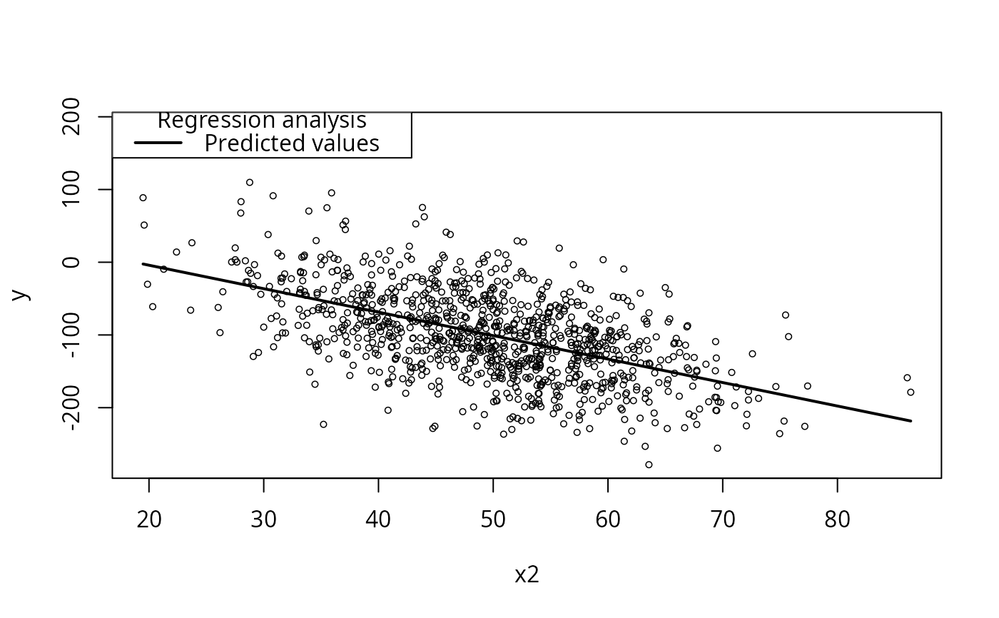
dat <- genCorrelatedData2(N = 1000, rho = 0,
beta = c(1, 0.2, -3.3, 1.1), stde = 50)
#> [1] "The equation that was calculated was"
#> y = 1 + 0.2*x1 + -3.3*x2 + 1.1*x3
#> + 0*x1*x1 + 0*x2*x1 + 0*x3*x1
#> + 0*x1*x2 + 0*x2*x2 + 0*x3*x2
#> + 0*x1*x3 + 0*x2*x3 + 0*x3*x3
#> + N(0,50) random error
m1 <- lm(y ~ x1 + x2 + x3, data = dat)
summary(m1)
#>
#> Call:
#> lm(formula = y ~ x1 + x2 + x3, data = dat)
#>
#> Residuals:
#> Min 1Q Median 3Q Max
#> -156.178 -33.319 -1.408 34.472 151.621
#>
#> Coefficients:
#> Estimate Std. Error t value Pr(>|t|)
#> (Intercept) -30.3746 13.3573 -2.274 0.0232 *
#> x1 0.3162 0.1600 1.976 0.0484 *
#> x2 -3.2270 0.1511 -21.354 <2e-16 ***
#> x3 1.4927 0.1533 9.734 <2e-16 ***
#> ---
#> Signif. codes: 0 ‘***’ 0.001 ‘**’ 0.01 ‘*’ 0.05 ‘.’ 0.1 ‘ ’ 1
#>
#> Residual standard error: 49.05 on 996 degrees of freedom
#> Multiple R-squared: 0.3507, Adjusted R-squared: 0.3487
#> F-statistic: 179.3 on 3 and 996 DF, p-value: < 2.2e-16
#>
predictOMatic(m1)
#> $x1
#> x1 x2 x3 fit
#> 1 19.06984 49.52024 50.22462 -109.17574
#> 2 43.34611 49.52024 50.22462 -101.50025
#> 3 50.07222 49.52024 50.22462 -99.37364
#> 4 56.53301 49.52024 50.22462 -97.33091
#> 5 80.78390 49.52024 50.22462 -89.66344
#>
#> $x2
#> x1 x2 x3 fit
#> 1 50.07666 19.48187 50.22462 -2.43962
#> 2 50.07666 42.66631 50.22462 -77.25489
#> 3 50.07666 49.93337 50.22462 -100.70537
#> 4 50.07666 56.80059 50.22462 -122.86562
#> 5 50.07666 86.38620 50.22462 -218.33718
#>
#> $x3
#> x1 x2 x3 fit
#> 1 50.07666 49.52024 9.411979 -160.29243
#> 2 50.07666 49.52024 43.753919 -109.03091
#> 3 50.07666 49.52024 50.158518 -99.47090
#> 4 50.07666 49.52024 56.718856 -89.67841
#> 5 50.07666 49.52024 87.543799 -43.66664
#>
plotCurves(m1, plotx = "x2")
 ## interaction between x1 and x2
dat <- genCorrelatedData2(N = 1000, rho = 0.2,
beta = c(1, 1.0, -1.1, 0.1, 0.0, 0.16), stde = 1)
#> [1] "The equation that was calculated was"
#> y = 1 + 1*x1 + -1.1*x2 + 0.1*x3
#> + 0*x1*x1 + 0.16*x2*x1 + 0*x3*x1
#> + 0*x1*x2 + 0*x2*x2 + 0*x3*x2
#> + 0*x1*x3 + 0*x2*x3 + 0*x3*x3
#> + N(0,1) random error
summarize(dat)
#> Numeric variables
#> y x1 x2 x3
#> min 110.848 21.979 13.727 12.388
#> med 391.626 49.933 50.001 50.515
#> max 850.418 81.294 91.046 90.485
#> mean 404.632 50.191 49.849 50.337
#> sd 128.111 10.169 10.257 9.800
#> skewness 0.584 0.148 -0.051 -0.013
#> kurtosis 0.285 -0.047 -0.057 0.614
#> nobs 1000 1000 1000 1000
#> nmissing 0 0 0 0
## Fit wrong model? get "wrong" result
m2w <- lm(y ~ x1 + x2 + x3, data = dat)
summary(m2w)
#>
#> Call:
#> lm(formula = y ~ x1 + x2 + x3, data = dat)
#>
#> Residuals:
#> Min 1Q Median 3Q Max
#> -60.809 -7.078 -2.207 5.780 91.749
#>
#> Coefficients:
#> Estimate Std. Error t value Pr(>|t|)
#> (Intercept) -405.67745 3.89743 -104.088 <2e-16 ***
#> x1 9.14954 0.05312 172.250 <2e-16 ***
#> x2 6.93795 0.05369 129.212 <2e-16 ***
#> x3 0.10412 0.05602 1.859 0.0634 .
#> ---
#> Signif. codes: 0 ‘***’ 0.001 ‘**’ 0.01 ‘*’ 0.05 ‘.’ 0.1 ‘ ’ 1
#>
#> Residual standard error: 16.68 on 996 degrees of freedom
#> Multiple R-squared: 0.9831, Adjusted R-squared: 0.983
#> F-statistic: 1.931e+04 on 3 and 996 DF, p-value: < 2.2e-16
#>
## Include interaction
m2 <- lm(y ~ x1 * x2 + x3, data = dat)
summary(m2)
#>
#> Call:
#> lm(formula = y ~ x1 * x2 + x3, data = dat)
#>
#> Residuals:
#> Min 1Q Median 3Q Max
#> -3.0875 -0.6834 -0.0058 0.6825 3.4888
#>
#> Coefficients:
#> Estimate Std. Error t value Pr(>|t|)
#> (Intercept) 0.4245115 0.8226541 0.516 0.606
#> x1 1.0082416 0.0161164 62.560 <2e-16 ***
#> x2 -1.0869092 0.0159025 -68.348 <2e-16 ***
#> x3 0.0982755 0.0034220 28.718 <2e-16 ***
#> x1:x2 0.1598309 0.0003099 515.714 <2e-16 ***
#> ---
#> Signif. codes: 0 ‘***’ 0.001 ‘**’ 0.01 ‘*’ 0.05 ‘.’ 0.1 ‘ ’ 1
#>
#> Residual standard error: 1.019 on 995 degrees of freedom
#> Multiple R-squared: 0.9999, Adjusted R-squared: 0.9999
#> F-statistic: 3.949e+06 on 4 and 995 DF, p-value: < 2.2e-16
#>
dat <- genCorrelatedData2(N = 1000, rho = 0.2,
beta = c(1, 1.0, -1.1, 0.1, 0.0, 0.16), stde = 100)
#> [1] "The equation that was calculated was"
#> y = 1 + 1*x1 + -1.1*x2 + 0.1*x3
#> + 0*x1*x1 + 0.16*x2*x1 + 0*x3*x1
#> + 0*x1*x2 + 0*x2*x2 + 0*x3*x2
#> + 0*x1*x3 + 0*x2*x3 + 0*x3*x3
#> + N(0,100) random error
summarize(dat)
#> Numeric variables
#> y x1 x2 x3
#> min -100.171 18.726 17.035 18.898
#> med 395.021 50.127 49.936 49.886
#> max 961.558 86.001 83.099 79.712
#> mean 402.661 49.843 49.769 50.112
#> sd 161.044 10.002 9.660 9.813
#> skewness 0.239 -0.087 -0.076 -0.032
#> kurtosis -0.026 0.063 0.112 -0.137
#> nobs 1000 1000 1000 1000
#> nmissing 0 0 0 0
m2.2 <- lm(y ~ x1 * x2 + x3, data = dat)
summary(m2.2)
#>
#> Call:
#> lm(formula = y ~ x1 * x2 + x3, data = dat)
#>
#> Residuals:
#> Min 1Q Median 3Q Max
#> -321.23 -72.65 -4.68 71.36 374.24
#>
#> Coefficients:
#> Estimate Std. Error t value Pr(>|t|)
#> (Intercept) 21.13536 82.17730 0.257 0.797
#> x1 0.18027 1.65703 0.109 0.913
#> x2 -1.72708 1.64315 -1.051 0.293
#> x3 0.38857 0.34116 1.139 0.255
#> x1:x2 0.17535 0.03266 5.370 9.82e-08 ***
#> ---
#> Signif. codes: 0 ‘***’ 0.001 ‘**’ 0.01 ‘*’ 0.05 ‘.’ 0.1 ‘ ’ 1
#>
#> Residual standard error: 101.2 on 995 degrees of freedom
#> Multiple R-squared: 0.607, Adjusted R-squared: 0.6054
#> F-statistic: 384.2 on 4 and 995 DF, p-value: < 2.2e-16
#>
dat <- genCorrelatedData2(N = 1000, means = c(100, 200, 300, 100),
sds = 20, rho = c(0.2, 0.3, 0.1, 0, 0, 0),
beta = c(1, 1.0, -1.1, 0.1, 0.0, 0.16, 0, 0, 0.2, 0, 0, 1.1, 0, 0, 0.1),
stde = 200)
#> [1] "The equation that was calculated was"
#> y = 1 + 1*x1 + -1.1*x2 + 0.1*x3 + 0*x4
#> + 0.16*x1*x1 + 0*x2*x1 + 0*x3*x1 + 0.2*x4*x1
#> + 0*x1*x2 + 0*x2*x2 + 0*x3*x2 + 1.1*x4*x2
#> + 0*x1*x3 + 0*x2*x3 + 0*x3*x3 + 0*x4*x3
#> + 0*x1*x4 + 0*x2*x4 + 0*x3*x4 + 0.1*x4*x4
#> + N(0,200) random error
summarize(dat)
#> Numeric variables
#> y x1 x2 x3 x4
#> min 8473.689 33.027 132.697 242.010 38.323
#> med 26409.413 99.238 199.714 300.518 100.233
#> max 45161.967 173.662 257.646 361.157 151.716
#> mean 26514.452 99.073 199.075 300.115 100.083
#> sd 5881.506 20.308 19.497 19.976 19.789
#> skewness 0.150 -0.025 -0.066 0.007 -0.104
#> kurtosis -0.144 0.155 0.176 -0.065 -0.176
#> nobs 1000 1000 1000 1000 1000
#> nmissing 0 0 0 0 0
m2.3w <- lm(y ~ x1 + x2 + x3, data = dat)
summary(m2)
#>
#> Call:
#> lm(formula = y ~ x1 * x2 + x3, data = dat)
#>
#> Residuals:
#> Min 1Q Median 3Q Max
#> -3.0875 -0.6834 -0.0058 0.6825 3.4888
#>
#> Coefficients:
#> Estimate Std. Error t value Pr(>|t|)
#> (Intercept) 0.4245115 0.8226541 0.516 0.606
#> x1 1.0082416 0.0161164 62.560 <2e-16 ***
#> x2 -1.0869092 0.0159025 -68.348 <2e-16 ***
#> x3 0.0982755 0.0034220 28.718 <2e-16 ***
#> x1:x2 0.1598309 0.0003099 515.714 <2e-16 ***
#> ---
#> Signif. codes: 0 ‘***’ 0.001 ‘**’ 0.01 ‘*’ 0.05 ‘.’ 0.1 ‘ ’ 1
#>
#> Residual standard error: 1.019 on 995 degrees of freedom
#> Multiple R-squared: 0.9999, Adjusted R-squared: 0.9999
#> F-statistic: 3.949e+06 on 4 and 995 DF, p-value: < 2.2e-16
#>
m2.3 <- lm(y ~ x1 * x2 + x3, data = dat)
summary(m2.3)
#>
#> Call:
#> lm(formula = y ~ x1 * x2 + x3, data = dat)
#>
#> Residuals:
#> Min 1Q Median 3Q Max
#> -14627.4 -3486.1 -103.7 3444.8 15068.8
#>
#> Coefficients:
#> Estimate Std. Error t value Pr(>|t|)
#> (Intercept) 6089.3545 8415.0040 0.724 0.4695
#> x1 7.8217 79.1288 0.099 0.9213
#> x2 79.0944 40.3791 1.959 0.0504 .
#> x3 -9.3619 8.5595 -1.094 0.2743
#> x1:x2 0.3390 0.3954 0.857 0.3915
#> ---
#> Signif. codes: 0 ‘***’ 0.001 ‘**’ 0.01 ‘*’ 0.05 ‘.’ 0.1 ‘ ’ 1
#>
#> Residual standard error: 5125 on 995 degrees of freedom
#> Multiple R-squared: 0.2436, Adjusted R-squared: 0.2406
#> F-statistic: 80.13 on 4 and 995 DF, p-value: < 2.2e-16
#>
predictOMatic(m2.3)
#> $x1
#> x1 x2 x3 fit
#> 1 33.02651 199.0754 300.1147 21512.68
#> 2 85.81525 199.0754 300.1147 25488.22
#> 3 99.23847 199.0754 300.1147 26499.13
#> 4 113.18309 199.0754 300.1147 27549.30
#> 5 173.66155 199.0754 300.1147 32103.96
#>
#> $x2
#> x1 x2 x3 fit
#> 1 99.07325 132.6968 300.1147 19007.06
#> 2 99.07325 186.2039 300.1147 25036.31
#> 3 99.07325 199.7137 300.1147 26558.62
#> 4 99.07325 211.7662 300.1147 27916.71
#> 5 99.07325 257.6461 300.1147 33086.51
#>
#> $x3
#> x1 x2 x3 fit
#> 1 99.07325 199.0754 242.0095 27030.66
#> 2 99.07325 199.0754 286.3391 26615.65
#> 3 99.07325 199.0754 300.5176 26482.91
#> 4 99.07325 199.0754 313.4495 26361.84
#> 5 99.07325 199.0754 361.1574 25915.21
#>
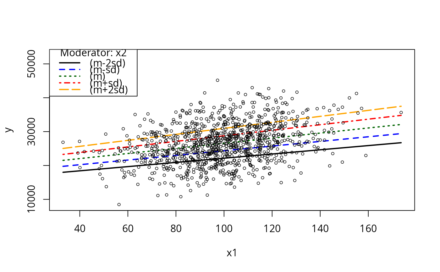
plotCurves(m2.3, plotx = "x1", modx = "x2", modxVals = "std.dev.", n = 5)
## interaction between x1 and x2
dat <- genCorrelatedData2(N = 1000, rho = 0.2,
beta = c(1, 1.0, -1.1, 0.1, 0.0, 0.16), stde = 1)
#> [1] "The equation that was calculated was"
#> y = 1 + 1*x1 + -1.1*x2 + 0.1*x3
#> + 0*x1*x1 + 0.16*x2*x1 + 0*x3*x1
#> + 0*x1*x2 + 0*x2*x2 + 0*x3*x2
#> + 0*x1*x3 + 0*x2*x3 + 0*x3*x3
#> + N(0,1) random error
summarize(dat)
#> Numeric variables
#> y x1 x2 x3
#> min 110.848 21.979 13.727 12.388
#> med 391.626 49.933 50.001 50.515
#> max 850.418 81.294 91.046 90.485
#> mean 404.632 50.191 49.849 50.337
#> sd 128.111 10.169 10.257 9.800
#> skewness 0.584 0.148 -0.051 -0.013
#> kurtosis 0.285 -0.047 -0.057 0.614
#> nobs 1000 1000 1000 1000
#> nmissing 0 0 0 0
## Fit wrong model? get "wrong" result
m2w <- lm(y ~ x1 + x2 + x3, data = dat)
summary(m2w)
#>
#> Call:
#> lm(formula = y ~ x1 + x2 + x3, data = dat)
#>
#> Residuals:
#> Min 1Q Median 3Q Max
#> -60.809 -7.078 -2.207 5.780 91.749
#>
#> Coefficients:
#> Estimate Std. Error t value Pr(>|t|)
#> (Intercept) -405.67745 3.89743 -104.088 <2e-16 ***
#> x1 9.14954 0.05312 172.250 <2e-16 ***
#> x2 6.93795 0.05369 129.212 <2e-16 ***
#> x3 0.10412 0.05602 1.859 0.0634 .
#> ---
#> Signif. codes: 0 ‘***’ 0.001 ‘**’ 0.01 ‘*’ 0.05 ‘.’ 0.1 ‘ ’ 1
#>
#> Residual standard error: 16.68 on 996 degrees of freedom
#> Multiple R-squared: 0.9831, Adjusted R-squared: 0.983
#> F-statistic: 1.931e+04 on 3 and 996 DF, p-value: < 2.2e-16
#>
## Include interaction
m2 <- lm(y ~ x1 * x2 + x3, data = dat)
summary(m2)
#>
#> Call:
#> lm(formula = y ~ x1 * x2 + x3, data = dat)
#>
#> Residuals:
#> Min 1Q Median 3Q Max
#> -3.0875 -0.6834 -0.0058 0.6825 3.4888
#>
#> Coefficients:
#> Estimate Std. Error t value Pr(>|t|)
#> (Intercept) 0.4245115 0.8226541 0.516 0.606
#> x1 1.0082416 0.0161164 62.560 <2e-16 ***
#> x2 -1.0869092 0.0159025 -68.348 <2e-16 ***
#> x3 0.0982755 0.0034220 28.718 <2e-16 ***
#> x1:x2 0.1598309 0.0003099 515.714 <2e-16 ***
#> ---
#> Signif. codes: 0 ‘***’ 0.001 ‘**’ 0.01 ‘*’ 0.05 ‘.’ 0.1 ‘ ’ 1
#>
#> Residual standard error: 1.019 on 995 degrees of freedom
#> Multiple R-squared: 0.9999, Adjusted R-squared: 0.9999
#> F-statistic: 3.949e+06 on 4 and 995 DF, p-value: < 2.2e-16
#>
dat <- genCorrelatedData2(N = 1000, rho = 0.2,
beta = c(1, 1.0, -1.1, 0.1, 0.0, 0.16), stde = 100)
#> [1] "The equation that was calculated was"
#> y = 1 + 1*x1 + -1.1*x2 + 0.1*x3
#> + 0*x1*x1 + 0.16*x2*x1 + 0*x3*x1
#> + 0*x1*x2 + 0*x2*x2 + 0*x3*x2
#> + 0*x1*x3 + 0*x2*x3 + 0*x3*x3
#> + N(0,100) random error
summarize(dat)
#> Numeric variables
#> y x1 x2 x3
#> min -100.171 18.726 17.035 18.898
#> med 395.021 50.127 49.936 49.886
#> max 961.558 86.001 83.099 79.712
#> mean 402.661 49.843 49.769 50.112
#> sd 161.044 10.002 9.660 9.813
#> skewness 0.239 -0.087 -0.076 -0.032
#> kurtosis -0.026 0.063 0.112 -0.137
#> nobs 1000 1000 1000 1000
#> nmissing 0 0 0 0
m2.2 <- lm(y ~ x1 * x2 + x3, data = dat)
summary(m2.2)
#>
#> Call:
#> lm(formula = y ~ x1 * x2 + x3, data = dat)
#>
#> Residuals:
#> Min 1Q Median 3Q Max
#> -321.23 -72.65 -4.68 71.36 374.24
#>
#> Coefficients:
#> Estimate Std. Error t value Pr(>|t|)
#> (Intercept) 21.13536 82.17730 0.257 0.797
#> x1 0.18027 1.65703 0.109 0.913
#> x2 -1.72708 1.64315 -1.051 0.293
#> x3 0.38857 0.34116 1.139 0.255
#> x1:x2 0.17535 0.03266 5.370 9.82e-08 ***
#> ---
#> Signif. codes: 0 ‘***’ 0.001 ‘**’ 0.01 ‘*’ 0.05 ‘.’ 0.1 ‘ ’ 1
#>
#> Residual standard error: 101.2 on 995 degrees of freedom
#> Multiple R-squared: 0.607, Adjusted R-squared: 0.6054
#> F-statistic: 384.2 on 4 and 995 DF, p-value: < 2.2e-16
#>
dat <- genCorrelatedData2(N = 1000, means = c(100, 200, 300, 100),
sds = 20, rho = c(0.2, 0.3, 0.1, 0, 0, 0),
beta = c(1, 1.0, -1.1, 0.1, 0.0, 0.16, 0, 0, 0.2, 0, 0, 1.1, 0, 0, 0.1),
stde = 200)
#> [1] "The equation that was calculated was"
#> y = 1 + 1*x1 + -1.1*x2 + 0.1*x3 + 0*x4
#> + 0.16*x1*x1 + 0*x2*x1 + 0*x3*x1 + 0.2*x4*x1
#> + 0*x1*x2 + 0*x2*x2 + 0*x3*x2 + 1.1*x4*x2
#> + 0*x1*x3 + 0*x2*x3 + 0*x3*x3 + 0*x4*x3
#> + 0*x1*x4 + 0*x2*x4 + 0*x3*x4 + 0.1*x4*x4
#> + N(0,200) random error
summarize(dat)
#> Numeric variables
#> y x1 x2 x3 x4
#> min 8473.689 33.027 132.697 242.010 38.323
#> med 26409.413 99.238 199.714 300.518 100.233
#> max 45161.967 173.662 257.646 361.157 151.716
#> mean 26514.452 99.073 199.075 300.115 100.083
#> sd 5881.506 20.308 19.497 19.976 19.789
#> skewness 0.150 -0.025 -0.066 0.007 -0.104
#> kurtosis -0.144 0.155 0.176 -0.065 -0.176
#> nobs 1000 1000 1000 1000 1000
#> nmissing 0 0 0 0 0
m2.3w <- lm(y ~ x1 + x2 + x3, data = dat)
summary(m2)
#>
#> Call:
#> lm(formula = y ~ x1 * x2 + x3, data = dat)
#>
#> Residuals:
#> Min 1Q Median 3Q Max
#> -3.0875 -0.6834 -0.0058 0.6825 3.4888
#>
#> Coefficients:
#> Estimate Std. Error t value Pr(>|t|)
#> (Intercept) 0.4245115 0.8226541 0.516 0.606
#> x1 1.0082416 0.0161164 62.560 <2e-16 ***
#> x2 -1.0869092 0.0159025 -68.348 <2e-16 ***
#> x3 0.0982755 0.0034220 28.718 <2e-16 ***
#> x1:x2 0.1598309 0.0003099 515.714 <2e-16 ***
#> ---
#> Signif. codes: 0 ‘***’ 0.001 ‘**’ 0.01 ‘*’ 0.05 ‘.’ 0.1 ‘ ’ 1
#>
#> Residual standard error: 1.019 on 995 degrees of freedom
#> Multiple R-squared: 0.9999, Adjusted R-squared: 0.9999
#> F-statistic: 3.949e+06 on 4 and 995 DF, p-value: < 2.2e-16
#>
m2.3 <- lm(y ~ x1 * x2 + x3, data = dat)
summary(m2.3)
#>
#> Call:
#> lm(formula = y ~ x1 * x2 + x3, data = dat)
#>
#> Residuals:
#> Min 1Q Median 3Q Max
#> -14627.4 -3486.1 -103.7 3444.8 15068.8
#>
#> Coefficients:
#> Estimate Std. Error t value Pr(>|t|)
#> (Intercept) 6089.3545 8415.0040 0.724 0.4695
#> x1 7.8217 79.1288 0.099 0.9213
#> x2 79.0944 40.3791 1.959 0.0504 .
#> x3 -9.3619 8.5595 -1.094 0.2743
#> x1:x2 0.3390 0.3954 0.857 0.3915
#> ---
#> Signif. codes: 0 ‘***’ 0.001 ‘**’ 0.01 ‘*’ 0.05 ‘.’ 0.1 ‘ ’ 1
#>
#> Residual standard error: 5125 on 995 degrees of freedom
#> Multiple R-squared: 0.2436, Adjusted R-squared: 0.2406
#> F-statistic: 80.13 on 4 and 995 DF, p-value: < 2.2e-16
#>
predictOMatic(m2.3)
#> $x1
#> x1 x2 x3 fit
#> 1 33.02651 199.0754 300.1147 21512.68
#> 2 85.81525 199.0754 300.1147 25488.22
#> 3 99.23847 199.0754 300.1147 26499.13
#> 4 113.18309 199.0754 300.1147 27549.30
#> 5 173.66155 199.0754 300.1147 32103.96
#>
#> $x2
#> x1 x2 x3 fit
#> 1 99.07325 132.6968 300.1147 19007.06
#> 2 99.07325 186.2039 300.1147 25036.31
#> 3 99.07325 199.7137 300.1147 26558.62
#> 4 99.07325 211.7662 300.1147 27916.71
#> 5 99.07325 257.6461 300.1147 33086.51
#>
#> $x3
#> x1 x2 x3 fit
#> 1 99.07325 199.0754 242.0095 27030.66
#> 2 99.07325 199.0754 286.3391 26615.65
#> 3 99.07325 199.0754 300.5176 26482.91
#> 4 99.07325 199.0754 313.4495 26361.84
#> 5 99.07325 199.0754 361.1574 25915.21
#>
plotCurves(m2.3, plotx = "x1", modx = "x2", modxVals = "std.dev.", n = 5)
 simReg <- lapply(1:100, function(x){
dat <- genCorrelatedData2(N = 1000, rho = c(0.2),
beta = c(1, 1.0, -1.1, 0.1, 0.0, 0.46), verbose = FALSE)
mymod <- lm (y ~ x1 * x2 + x3, data = dat)
summary(mymod)
})
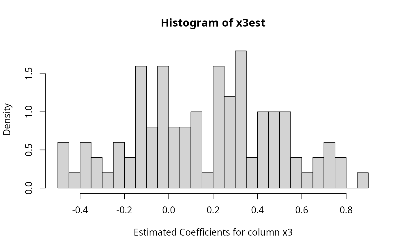
x3est <- sapply(simReg, function(reg) {coef(reg)[4 ,1] })
summarize(x3est)
#> Numeric variables
#> x3est
#> min -0.495
#> med 0.205
#> max 0.874
#> mean 0.167
#> sd 0.321
#> skewness -0.006
#> kurtosis -0.749
#> nobs 100
#> nmissing 0
hist(x3est, breaks = 40, prob = TRUE,
xlab = "Estimated Coefficients for column x3")
simReg <- lapply(1:100, function(x){
dat <- genCorrelatedData2(N = 1000, rho = c(0.2),
beta = c(1, 1.0, -1.1, 0.1, 0.0, 0.46), verbose = FALSE)
mymod <- lm (y ~ x1 * x2 + x3, data = dat)
summary(mymod)
})
x3est <- sapply(simReg, function(reg) {coef(reg)[4 ,1] })
summarize(x3est)
#> Numeric variables
#> x3est
#> min -0.495
#> med 0.205
#> max 0.874
#> mean 0.167
#> sd 0.321
#> skewness -0.006
#> kurtosis -0.749
#> nobs 100
#> nmissing 0
hist(x3est, breaks = 40, prob = TRUE,
xlab = "Estimated Coefficients for column x3")
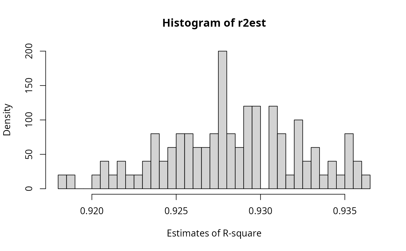
 r2est <- sapply(simReg, function(reg) {reg$r.square})
summarize(r2est)
#> Numeric variables
#> r2est
#> min 0.918
#> med 0.928
#> max 0.936
#> mean 0.928
#> sd 0.004
#> skewness -0.148
#> kurtosis -0.509
#> nobs 100
#> nmissing 0
hist(r2est, breaks = 40, prob = TRUE, xlab = "Estimates of R-square")
r2est <- sapply(simReg, function(reg) {reg$r.square})
summarize(r2est)
#> Numeric variables
#> r2est
#> min 0.918
#> med 0.928
#> max 0.936
#> mean 0.928
#> sd 0.004
#> skewness -0.148
#> kurtosis -0.509
#> nobs 100
#> nmissing 0
hist(r2est, breaks = 40, prob = TRUE, xlab = "Estimates of R-square")
 ## No interaction, collinearity
dat <- genCorrelatedData2(N = 1000, rho = c(0.1, 0.2, 0.7),
beta = c(1, 1.0, -1.1, 0.1), stde = 1)
#> [1] "The equation that was calculated was"
#> y = 1 + 1*x1 + -1.1*x2 + 0.1*x3
#> + 0*x1*x1 + 0*x2*x1 + 0*x3*x1
#> + 0*x1*x2 + 0*x2*x2 + 0*x3*x2
#> + 0*x1*x3 + 0*x2*x3 + 0*x3*x3
#> + N(0,1) random error
m3 <- lm(y ~ x1 + x2 + x3, data = dat)
summary(m3)
#>
#> Call:
#> lm(formula = y ~ x1 + x2 + x3, data = dat)
#>
#> Residuals:
#> Min 1Q Median 3Q Max
#> -3.4238 -0.6451 -0.0207 0.6719 3.3106
#>
#> Coefficients:
#> Estimate Std. Error t value Pr(>|t|)
#> (Intercept) 1.128194 0.214071 5.27 1.67e-07 ***
#> x1 0.998219 0.003170 314.86 < 2e-16 ***
#> x2 -1.096284 0.004482 -244.57 < 2e-16 ***
#> x3 0.096807 0.004528 21.38 < 2e-16 ***
#> ---
#> Signif. codes: 0 ‘***’ 0.001 ‘**’ 0.01 ‘*’ 0.05 ‘.’ 0.1 ‘ ’ 1
#>
#> Residual standard error: 0.9881 on 996 degrees of freedom
#> Multiple R-squared: 0.9948, Adjusted R-squared: 0.9948
#> F-statistic: 6.377e+04 on 3 and 996 DF, p-value: < 2.2e-16
#>
dat <- genCorrelatedData2(N=1000, rho=c(0.1, 0.2, 0.7),
beta = c(1, 1.0, -1.1, 0.1), stde = 200)
#> [1] "The equation that was calculated was"
#> y = 1 + 1*x1 + -1.1*x2 + 0.1*x3
#> + 0*x1*x1 + 0*x2*x1 + 0*x3*x1
#> + 0*x1*x2 + 0*x2*x2 + 0*x3*x2
#> + 0*x1*x3 + 0*x2*x3 + 0*x3*x3
#> + N(0,200) random error
m3 <- lm(y ~ x1 + x2 + x3, data = dat)
summary(m3)
#>
#> Call:
#> lm(formula = y ~ x1 + x2 + x3, data = dat)
#>
#> Residuals:
#> Min 1Q Median 3Q Max
#> -604.75 -139.76 -2.97 136.72 714.60
#>
#> Coefficients:
#> Estimate Std. Error t value Pr(>|t|)
#> (Intercept) -18.3289 44.2699 -0.414 0.6789
#> x1 1.3780 0.6628 2.079 0.0379 *
#> x2 -0.8842 0.9115 -0.970 0.3323
#> x3 -0.1108 0.8888 -0.125 0.9008
#> ---
#> Signif. codes: 0 ‘***’ 0.001 ‘**’ 0.01 ‘*’ 0.05 ‘.’ 0.1 ‘ ’ 1
#>
#> Residual standard error: 196.4 on 996 degrees of freedom
#> Multiple R-squared: 0.006149, Adjusted R-squared: 0.003156
#> F-statistic: 2.054 on 3 and 996 DF, p-value: 0.1047
#>
mcDiagnose(m3)
#> The following auxiliary models are being estimated and returned in a list:
#> x1 ~ x2 + x3
#> x2 ~ x1 + x3
#> x3 ~ x1 + x2
#>
#> R_j Squares of auxiliary models
#> x1 x2 x3
#> 0.04268692 0.51630974 0.53071812
#> The Corresponding VIF, 1/(1-R_j^2)
#> x1 x2 x3
#> 1.044590 2.067439 2.130915
#> Bivariate Pearson Correlations for design matrix
#> x1 x2 x3
#> x1 1.00 0.09 0.19
#> x2 0.09 1.00 0.72
#> x3 0.19 0.72 1.00
dat <- genCorrelatedData2(N = 1000, rho = c(0.9, 0.5, 0.4),
beta = c(1, 1.0, -1.1, 0.1), stde = 200)
#> [1] "The equation that was calculated was"
#> y = 1 + 1*x1 + -1.1*x2 + 0.1*x3
#> + 0*x1*x1 + 0*x2*x1 + 0*x3*x1
#> + 0*x1*x2 + 0*x2*x2 + 0*x3*x2
#> + 0*x1*x3 + 0*x2*x3 + 0*x3*x3
#> + N(0,200) random error
m3b <- lm(y ~ x1 + x2 + x3, data = dat)
summary(m3b)
#>
#> Call:
#> lm(formula = y ~ x1 + x2 + x3, data = dat)
#>
#> Residuals:
#> Min 1Q Median 3Q Max
#> -570.60 -147.86 -2.39 137.17 638.03
#>
#> Coefficients:
#> Estimate Std. Error t value Pr(>|t|)
#> (Intercept) 17.045637 39.825486 0.428 0.669
#> x1 -0.005261 1.565198 -0.003 0.997
#> x2 -0.997605 1.479232 -0.674 0.500
#> x3 0.665004 0.773560 0.860 0.390
#>
#> Residual standard error: 205.3 on 996 degrees of freedom
#> Multiple R-squared: 0.002128, Adjusted R-squared: -0.0008776
#> F-statistic: 0.708 on 3 and 996 DF, p-value: 0.5473
#>
mcDiagnose(m3b)
#> The following auxiliary models are being estimated and returned in a list:
#> x1 ~ x2 + x3
#> x2 ~ x1 + x3
#> x3 ~ x1 + x2
#>
#> R_j Squares of auxiliary models
#> x1 x2 x3
#> 0.8288619 0.8082557 0.2687030
#> The Corresponding VIF, 1/(1-R_j^2)
#> x1 x2 x3
#> 5.843236 5.215279 1.367433
#> Bivariate Pearson Correlations for design matrix
#> x1 x2 x3
#> x1 1.00 0.90 0.51
#> x2 0.90 1.00 0.41
#> x3 0.51 0.41 1.00
## No interaction, collinearity
dat <- genCorrelatedData2(N = 1000, rho = c(0.1, 0.2, 0.7),
beta = c(1, 1.0, -1.1, 0.1), stde = 1)
#> [1] "The equation that was calculated was"
#> y = 1 + 1*x1 + -1.1*x2 + 0.1*x3
#> + 0*x1*x1 + 0*x2*x1 + 0*x3*x1
#> + 0*x1*x2 + 0*x2*x2 + 0*x3*x2
#> + 0*x1*x3 + 0*x2*x3 + 0*x3*x3
#> + N(0,1) random error
m3 <- lm(y ~ x1 + x2 + x3, data = dat)
summary(m3)
#>
#> Call:
#> lm(formula = y ~ x1 + x2 + x3, data = dat)
#>
#> Residuals:
#> Min 1Q Median 3Q Max
#> -3.4238 -0.6451 -0.0207 0.6719 3.3106
#>
#> Coefficients:
#> Estimate Std. Error t value Pr(>|t|)
#> (Intercept) 1.128194 0.214071 5.27 1.67e-07 ***
#> x1 0.998219 0.003170 314.86 < 2e-16 ***
#> x2 -1.096284 0.004482 -244.57 < 2e-16 ***
#> x3 0.096807 0.004528 21.38 < 2e-16 ***
#> ---
#> Signif. codes: 0 ‘***’ 0.001 ‘**’ 0.01 ‘*’ 0.05 ‘.’ 0.1 ‘ ’ 1
#>
#> Residual standard error: 0.9881 on 996 degrees of freedom
#> Multiple R-squared: 0.9948, Adjusted R-squared: 0.9948
#> F-statistic: 6.377e+04 on 3 and 996 DF, p-value: < 2.2e-16
#>
dat <- genCorrelatedData2(N=1000, rho=c(0.1, 0.2, 0.7),
beta = c(1, 1.0, -1.1, 0.1), stde = 200)
#> [1] "The equation that was calculated was"
#> y = 1 + 1*x1 + -1.1*x2 + 0.1*x3
#> + 0*x1*x1 + 0*x2*x1 + 0*x3*x1
#> + 0*x1*x2 + 0*x2*x2 + 0*x3*x2
#> + 0*x1*x3 + 0*x2*x3 + 0*x3*x3
#> + N(0,200) random error
m3 <- lm(y ~ x1 + x2 + x3, data = dat)
summary(m3)
#>
#> Call:
#> lm(formula = y ~ x1 + x2 + x3, data = dat)
#>
#> Residuals:
#> Min 1Q Median 3Q Max
#> -604.75 -139.76 -2.97 136.72 714.60
#>
#> Coefficients:
#> Estimate Std. Error t value Pr(>|t|)
#> (Intercept) -18.3289 44.2699 -0.414 0.6789
#> x1 1.3780 0.6628 2.079 0.0379 *
#> x2 -0.8842 0.9115 -0.970 0.3323
#> x3 -0.1108 0.8888 -0.125 0.9008
#> ---
#> Signif. codes: 0 ‘***’ 0.001 ‘**’ 0.01 ‘*’ 0.05 ‘.’ 0.1 ‘ ’ 1
#>
#> Residual standard error: 196.4 on 996 degrees of freedom
#> Multiple R-squared: 0.006149, Adjusted R-squared: 0.003156
#> F-statistic: 2.054 on 3 and 996 DF, p-value: 0.1047
#>
mcDiagnose(m3)
#> The following auxiliary models are being estimated and returned in a list:
#> x1 ~ x2 + x3
#> x2 ~ x1 + x3
#> x3 ~ x1 + x2
#>
#> R_j Squares of auxiliary models
#> x1 x2 x3
#> 0.04268692 0.51630974 0.53071812
#> The Corresponding VIF, 1/(1-R_j^2)
#> x1 x2 x3
#> 1.044590 2.067439 2.130915
#> Bivariate Pearson Correlations for design matrix
#> x1 x2 x3
#> x1 1.00 0.09 0.19
#> x2 0.09 1.00 0.72
#> x3 0.19 0.72 1.00
dat <- genCorrelatedData2(N = 1000, rho = c(0.9, 0.5, 0.4),
beta = c(1, 1.0, -1.1, 0.1), stde = 200)
#> [1] "The equation that was calculated was"
#> y = 1 + 1*x1 + -1.1*x2 + 0.1*x3
#> + 0*x1*x1 + 0*x2*x1 + 0*x3*x1
#> + 0*x1*x2 + 0*x2*x2 + 0*x3*x2
#> + 0*x1*x3 + 0*x2*x3 + 0*x3*x3
#> + N(0,200) random error
m3b <- lm(y ~ x1 + x2 + x3, data = dat)
summary(m3b)
#>
#> Call:
#> lm(formula = y ~ x1 + x2 + x3, data = dat)
#>
#> Residuals:
#> Min 1Q Median 3Q Max
#> -570.60 -147.86 -2.39 137.17 638.03
#>
#> Coefficients:
#> Estimate Std. Error t value Pr(>|t|)
#> (Intercept) 17.045637 39.825486 0.428 0.669
#> x1 -0.005261 1.565198 -0.003 0.997
#> x2 -0.997605 1.479232 -0.674 0.500
#> x3 0.665004 0.773560 0.860 0.390
#>
#> Residual standard error: 205.3 on 996 degrees of freedom
#> Multiple R-squared: 0.002128, Adjusted R-squared: -0.0008776
#> F-statistic: 0.708 on 3 and 996 DF, p-value: 0.5473
#>
mcDiagnose(m3b)
#> The following auxiliary models are being estimated and returned in a list:
#> x1 ~ x2 + x3
#> x2 ~ x1 + x3
#> x3 ~ x1 + x2
#>
#> R_j Squares of auxiliary models
#> x1 x2 x3
#> 0.8288619 0.8082557 0.2687030
#> The Corresponding VIF, 1/(1-R_j^2)
#> x1 x2 x3
#> 5.843236 5.215279 1.367433
#> Bivariate Pearson Correlations for design matrix
#> x1 x2 x3
#> x1 1.00 0.90 0.51
#> x2 0.90 1.00 0.41
#> x3 0.51 0.41 1.00