Hypothesis tests for Simple Slopes Objects
testSlopes.RdConducts t-test of the hypothesis that the "simple slope" line for
one predictor is statistically significantly different from zero
for each value of a moderator variable. The user must first run
plotSlopes(), and then give the output object to
plotSlopes(). A plot method has been implemented for
testSlopes objects. It will create an interesting display, but
only when the moderator is a numeric variable.
Value
A list including 1) the hypothesis test table, 2) a copy of the plotSlopes object, and, for numeric modx variables, 3) the Johnson-Neyman (J-N) interval boundaries.
Details
This function scans the input object to detect the focal values of
the moderator variable (the variable declared as modx in
plotSlopes). Consider a regression with interactions
y <- b0 + b1*x1 + b2*x2 + b3*(x1*x2) + b4*x3 + ... + error
If plotSlopes has been run with the argument plotx="x1" and
the argument modx="x2", then there will be several plotted lines,
one for each of the chosen values of x2. The slope of each of
these lines depends on x1's effect, b1, as well as the interactive
part, b3*x2.
This function performs a test of the null hypothesis of the slope
of each fitted line in a plotSlopes object is statistically
significant from zero. A simple t-test for each line is offered.
No correction for the conduct of multiple hypothesis tests (no
Bonferroni correction).
When modx is a numeric variable, it is possible to conduct
further analysis. We ask "for which values of modx would
the effect of plotx be statistically significant?" This is
called a Johnson-Neyman (Johnson-Neyman, 1936) approach in
Preacher, Curran, and Bauer (2006). The interval is calculated
here. A plot method is provided to illustrate the result.
References
Preacher, Kristopher J, Curran, Patrick J.,and Bauer, Daniel J. (2006). Computational Tools for Probing Interactions in Multiple Linear Regression, Multilevel Modeling, and Latent Curve Analysis. Journal of Educational and Behavioral Statistics. 31,4, 437-448.
Johnson, P.O. and Neyman, J. (1936). "Tests of certain linear hypotheses and their applications to some educational problems. Statistical Research Memoirs, 1, 57-93.
Author
Paul E. Johnson pauljohn@ku.edu
Examples
library(rockchalk)
library(carData)
m1 <- lm(statusquo ~ income * age + education + sex + age, data = Chile)
m1ps <- plotSlopes(m1, modx = "income", plotx = "age")
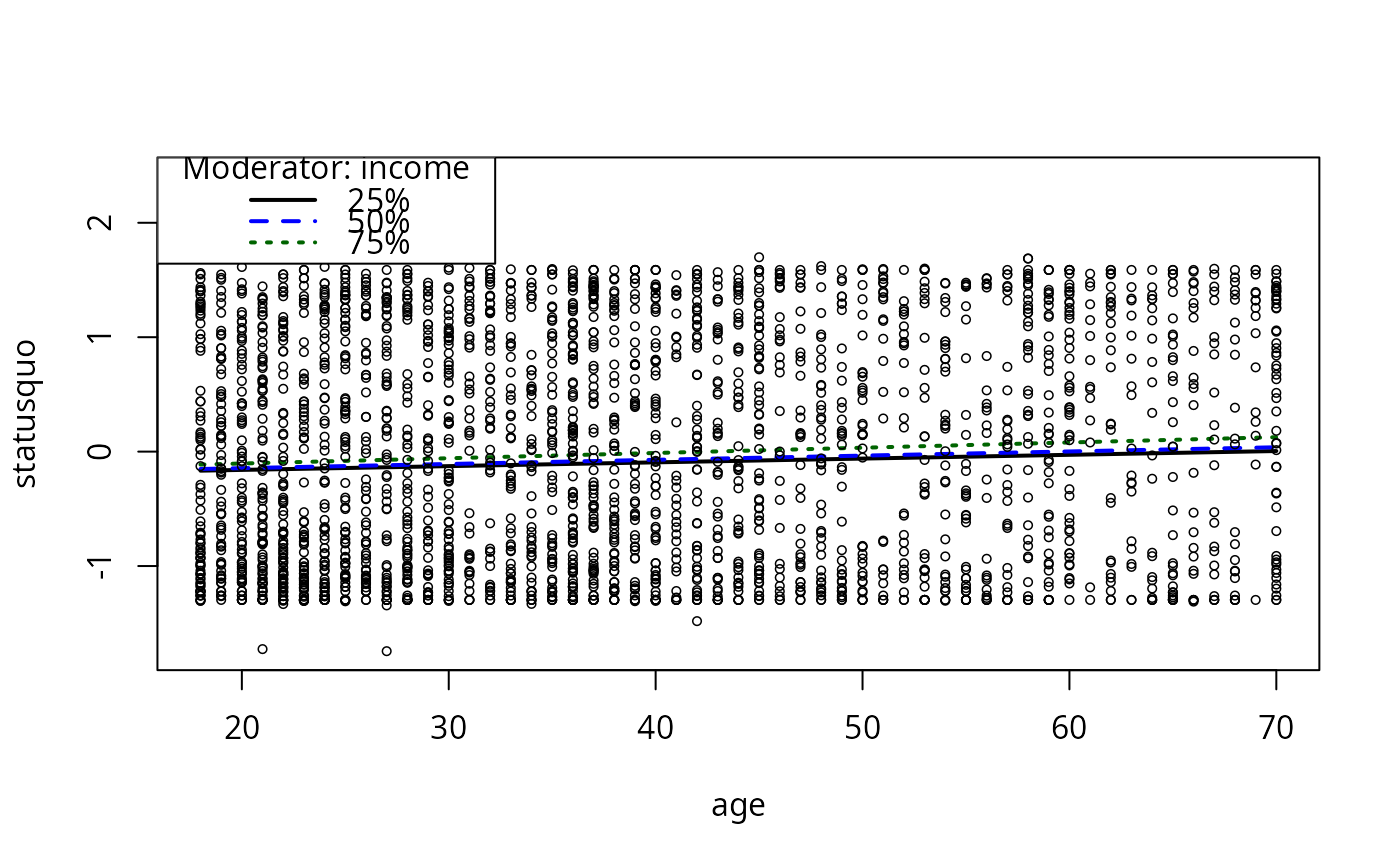 m1psts <- testSlopes(m1ps)
#> Error in eval(parse(text = object$call$model)): object 'm1' not found
plot(m1psts)
#> Error: object 'm1psts' not found
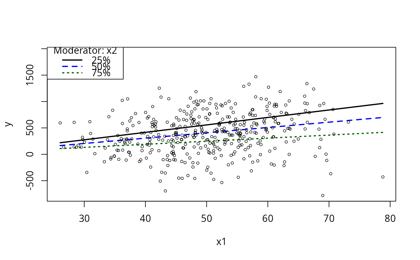
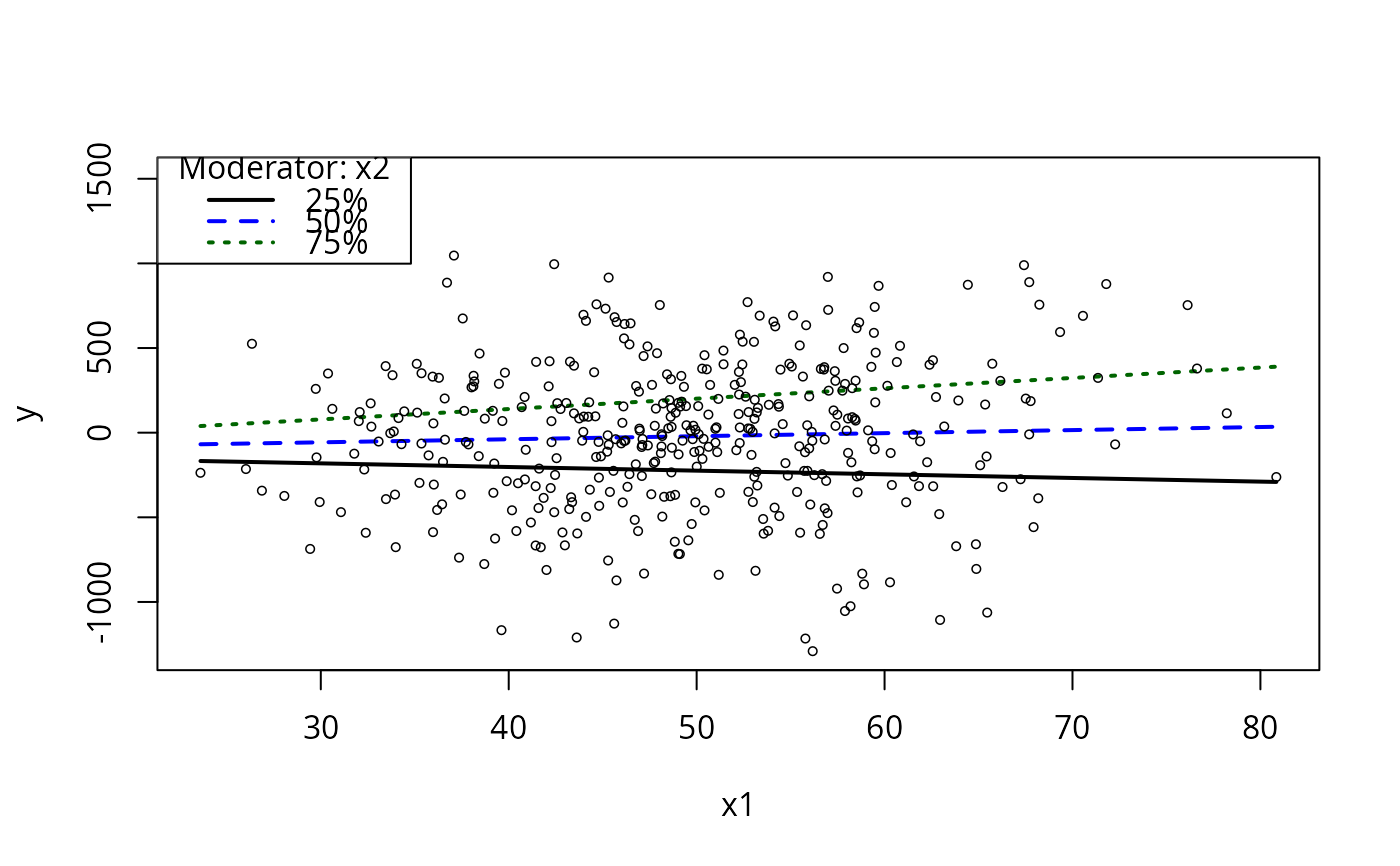
dat2 <- genCorrelatedData(N = 400, rho = .1, means = c(50, -20),
stde = 300, beta = c(2, 0, 0.1, -0.4))
m2 <- lm(y ~ x1*x2, data = dat2)
m2ps <- plotSlopes(m2, plotx = "x1", modx = "x2")
m1psts <- testSlopes(m1ps)
#> Error in eval(parse(text = object$call$model)): object 'm1' not found
plot(m1psts)
#> Error: object 'm1psts' not found
dat2 <- genCorrelatedData(N = 400, rho = .1, means = c(50, -20),
stde = 300, beta = c(2, 0, 0.1, -0.4))
m2 <- lm(y ~ x1*x2, data = dat2)
m2ps <- plotSlopes(m2, plotx = "x1", modx = "x2")
 m2psts <- testSlopes(m2ps)
#> Error in eval(parse(text = object$call$model)): object 'm2' not found
plot(m2psts)
#> Error: object 'm2psts' not found
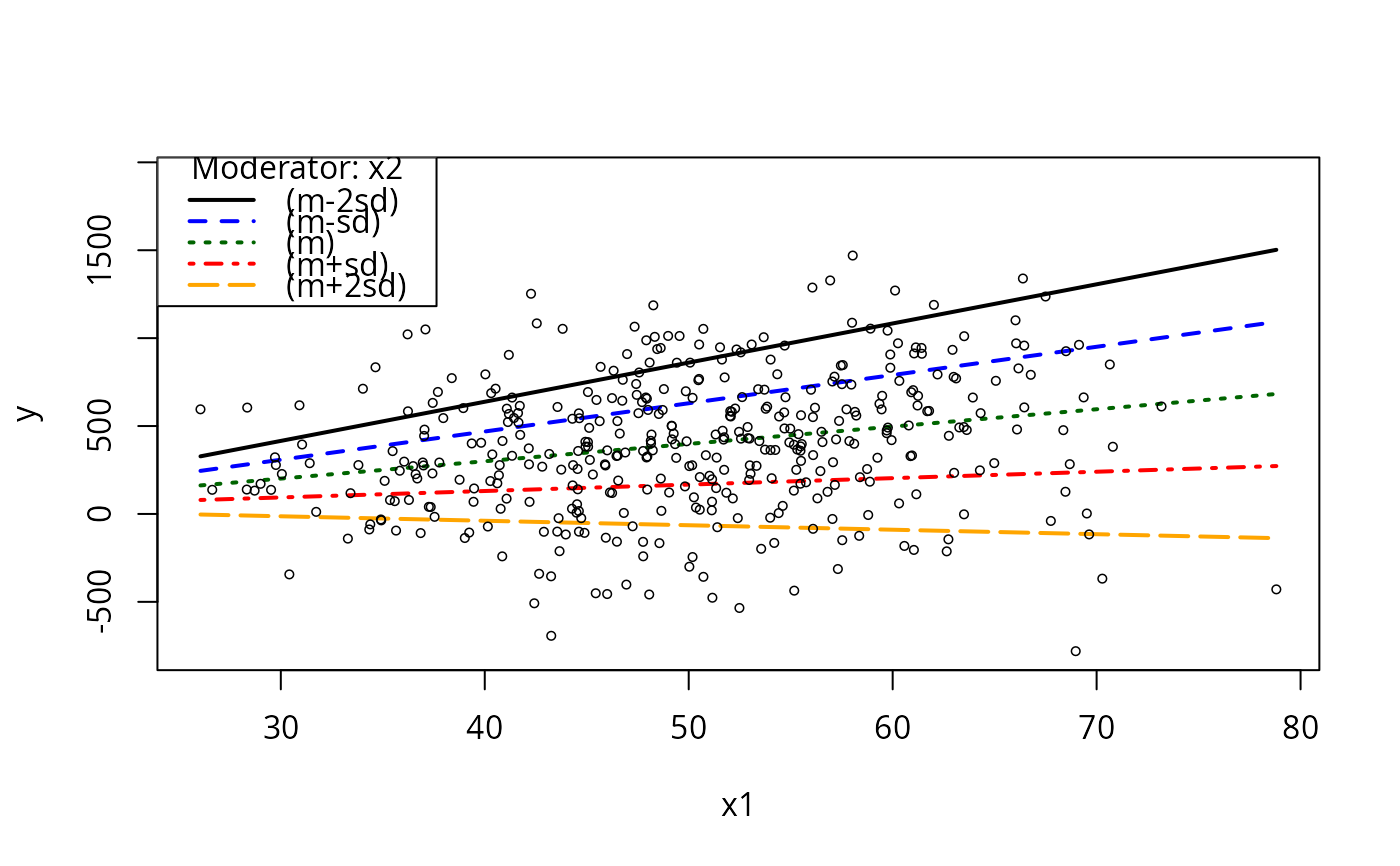
m2ps <- plotSlopes(m2, plotx = "x1", modx = "x2", modxVals = "std.dev", n = 5)
m2psts <- testSlopes(m2ps)
#> Error in eval(parse(text = object$call$model)): object 'm2' not found
plot(m2psts)
#> Error: object 'm2psts' not found
m2ps <- plotSlopes(m2, plotx = "x1", modx = "x2", modxVals = "std.dev", n = 5)
 m2psts <- testSlopes(m2ps)
#> Error in eval(parse(text = object$call$model)): object 'm2' not found
plot(m2psts)
#> Error: object 'm2psts' not found
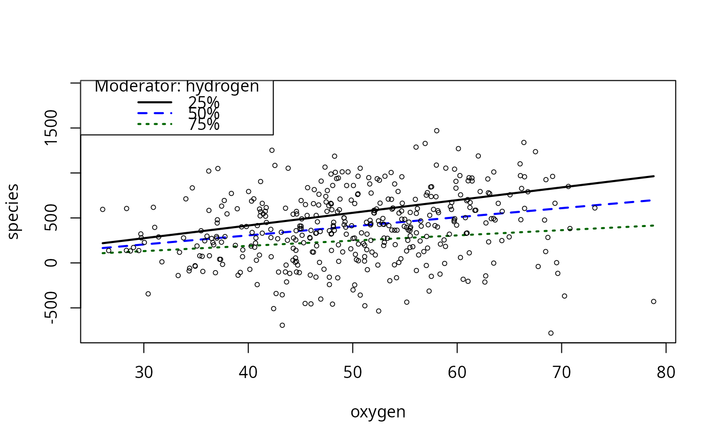
## Try again with longer variable names
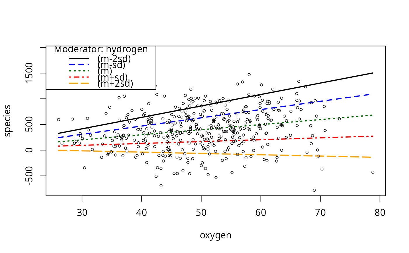
colnames(dat2) <- c("oxygen","hydrogen","species")
m2a <- lm(species ~ oxygen*hydrogen, data = dat2)
m2aps1 <- plotSlopes(m2a, plotx = "oxygen", modx = "hydrogen")
m2psts <- testSlopes(m2ps)
#> Error in eval(parse(text = object$call$model)): object 'm2' not found
plot(m2psts)
#> Error: object 'm2psts' not found
## Try again with longer variable names
colnames(dat2) <- c("oxygen","hydrogen","species")
m2a <- lm(species ~ oxygen*hydrogen, data = dat2)
m2aps1 <- plotSlopes(m2a, plotx = "oxygen", modx = "hydrogen")
 m2aps1ts <- testSlopes(m2aps1)
#> Error in eval(parse(text = object$call$model)): object 'm2a' not found
plot(m2aps1ts)
#> Error: object 'm2aps1ts' not found
m2aps2 <- plotSlopes(m2a, plotx = "oxygen", modx = "hydrogen",
modxVals = "std.dev", n = 5)
m2aps1ts <- testSlopes(m2aps1)
#> Error in eval(parse(text = object$call$model)): object 'm2a' not found
plot(m2aps1ts)
#> Error: object 'm2aps1ts' not found
m2aps2 <- plotSlopes(m2a, plotx = "oxygen", modx = "hydrogen",
modxVals = "std.dev", n = 5)
 m2bps2ts <- testSlopes(m2aps2)
#> Error in eval(parse(text = object$call$model)): object 'm2a' not found
plot(m2bps2ts)
#> Error: object 'm2bps2ts' not found
dat3 <- genCorrelatedData(N = 400, rho = .1, stde = 300,
beta = c(2, 0, 0.3, 0.15),
means = c(50,0), sds = c(10, 40))
m3 <- lm(y ~ x1*x2, data = dat3)
m3ps <- plotSlopes(m3, plotx = "x1", modx = "x2")
m2bps2ts <- testSlopes(m2aps2)
#> Error in eval(parse(text = object$call$model)): object 'm2a' not found
plot(m2bps2ts)
#> Error: object 'm2bps2ts' not found
dat3 <- genCorrelatedData(N = 400, rho = .1, stde = 300,
beta = c(2, 0, 0.3, 0.15),
means = c(50,0), sds = c(10, 40))
m3 <- lm(y ~ x1*x2, data = dat3)
m3ps <- plotSlopes(m3, plotx = "x1", modx = "x2")
 m3sts <- testSlopes(m3ps)
#> Error in eval(parse(text = object$call$model)): object 'm3' not found
plot(testSlopes(m3ps))
#> Error in eval(parse(text = object$call$model)): object 'm3' not found
plot(testSlopes(m3ps), shade = FALSE)
#> Error in eval(parse(text = object$call$model)): object 'm3' not found
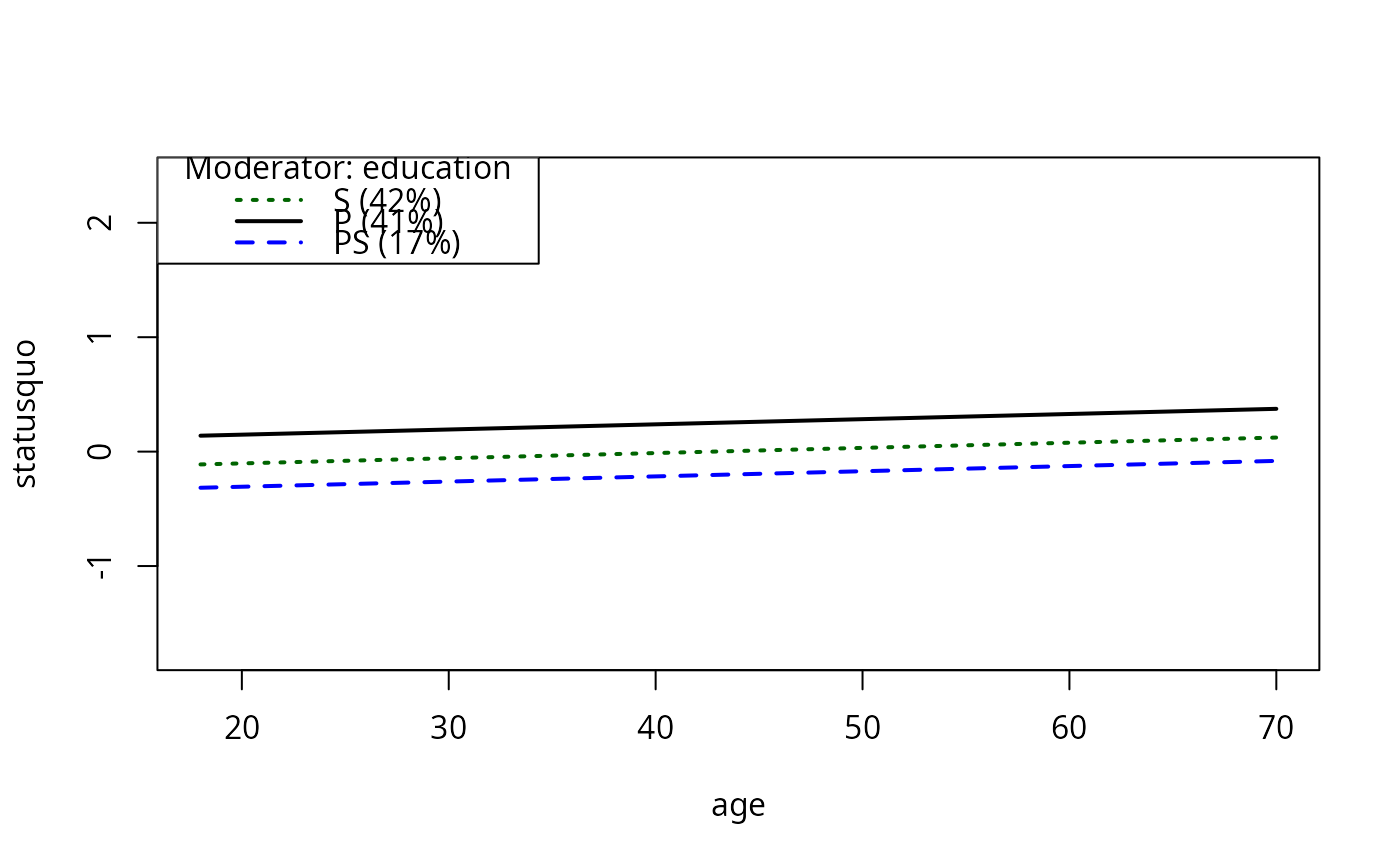
## Finally, if model has no relevant interactions, testSlopes does nothing.
m9 <- lm(statusquo ~ age + income * education + sex + age, data = Chile)
m9ps <- plotSlopes(m9, modx = "education", plotx = "age", plotPoints = FALSE)
m3sts <- testSlopes(m3ps)
#> Error in eval(parse(text = object$call$model)): object 'm3' not found
plot(testSlopes(m3ps))
#> Error in eval(parse(text = object$call$model)): object 'm3' not found
plot(testSlopes(m3ps), shade = FALSE)
#> Error in eval(parse(text = object$call$model)): object 'm3' not found
## Finally, if model has no relevant interactions, testSlopes does nothing.
m9 <- lm(statusquo ~ age + income * education + sex + age, data = Chile)
m9ps <- plotSlopes(m9, modx = "education", plotx = "age", plotPoints = FALSE)
 m9psts <- testSlopes(m9ps)
#> Error in eval(parse(text = object$call$model)): object 'm9' not found
m9psts <- testSlopes(m9ps)
#> Error in eval(parse(text = object$call$model)): object 'm9' not found