meanCenter
meanCenter.RdmeanCenter selectively centers or standarizes variables in a regression model.
Usage
meanCenter(
  model,
  centerOnlyInteractors = TRUE,
  centerDV = FALSE,
  standardize = FALSE,
  terms = NULL
)

# Default S3 method
meanCenter(
  model,
  centerOnlyInteractors = TRUE,
  centerDV = FALSE,
  standardize = FALSE,
  terms = NULL
)
Arguments
- model
a fitted regression model (presumably from lm)
- centerOnlyInteractors
Default TRUE. If FALSE, all numeric predictors in the regression data frame are centered before the regression is conducted.
- centerDV
Default FALSE. Should the dependent variable be centered? Do not set this option to TRUE unless the dependent variable is a numeric variable. Otherwise, it is an error.
- standardize
Default FALSE. Instead of simply mean-centering the variables, should they also be "standardized" by first mean-centering and then dividing by the estimated standard deviation.
- terms
Optional. A vector of variable names to be centered. Supplying this argument will stop meanCenter from searching for interaction terms that might need to be centered.
Value
A regression model of the same type as the input model, with attributes representing the names of the centered variables.
Details
Works with "lm" class objects, objects estimated by glm(). This
centers some or all of the the predictors and then re-fits the
original model with the new variables. This is a convenience to
researchers who are often urged to center their predictors. This
is sometimes suggested as a way to ameliorate multi-collinearity
in models that include interaction terms (Aiken and West, 1991;
Cohen, et al 2002). Mean-centering may enhance interpretation of
the regression intercept, but it actually does not help with
multicollinearity. (Echambadi and Hess, 2007). This function
facilitates comparison of mean-centered models with others by
calculating centered variables. The defaults will cause a
regression's numeric interactive variables to be mean
centered. Variations on the arguments are discussed in details.
Suppose the user's formula that fits the original model is
m1 <- lm(y ~ x1*x2 + x3 + x4, data = dat). The fitted model
will include estimates for predictors x1, x2,
x1:x2, x3 and x4. By default,
meanCenter(m1) scans the output to see if there are
interaction terms of the form x1:x2. If so, then x1 and x2
are replaced by centered versions (m1-mean(m1)) and
(m2-mean(m2)). The model is re-estimated with those new variables.
model (the main effect and the interaction). The resulting thing
is "just another regression model", which can be analyzed or
plotted like any R regression object.
The user can claim control over which variables are centered in
several ways. Most directly, by specifying a vector of variable
names, the user can claim direct control. For example, the
argument terms=c("x1","x2","x3") would cause 3 predictors
to be centered. If one wants all predictors to be centered, the
argument centerOnlyInteractors should be set to
FALSE. Please note, this WILL NOT center factor variables. But it
will find all numeric predictors and center them.
The dependent variable will not be centered, unless the user explicitly requests it by setting centerDV = TRUE.
As an additional convenience to the user, the argument
standardize = TRUE can be used. This will divide each
centered variable by its observed standard deviation. For people
who like standardized regression, I suggest this is a better
approach than the standardize function (which is brain-dead
in the style of SPSS). meanCenter with standardize = TRUE
will only try to standardize the numeric predictors.
To be completely clear, I believe mean-centering is not helpful with the multicollinearity problem. It doesn't help, it doesn't hurt. Only a misunderstanding leads its proponents to claim otherwise. This is emphasized in the vignette "rockchalk" that is distributed with this package.
References
Aiken, L. S. and West, S.G. (1991). Multiple Regression: Testing and Interpreting Interactions. Newbury Park, Calif: Sage Publications.
Cohen, J., Cohen, P., West, S. G., and Aiken, L. S. (2002). Applied Multiple Regression/Correlation Analysis for the Behavioral Sciences (Third.). Routledge Academic.
Echambadi, R., and Hess, J. D. (2007). Mean-Centering Does Not Alleviate Collinearity Problems in Moderated Multiple Regression Models. Marketing Science, 26(3), 438-445.
Author
Paul E. Johnson pauljohn@ku.edu
Examples
library(rockchalk)
N <- 100
dat <- genCorrelatedData(N = N, means = c(100, 200), sds = c(20, 30),
rho = 0.4, stde = 10)
dat$x3 <- rnorm(100, m = 40, s = 4)
m1 <- lm(y ~ x1 * x2 + x3, data = dat)
summary(m1)
#>
#> Call:
#> lm(formula = y ~ x1 * x2 + x3, data = dat)
#>
#> Residuals:
#> Min 1Q Median 3Q Max
#> -23.679 -4.835 0.081 6.131 22.732
#>
#> Coefficients:
#> Estimate Std. Error t value Pr(>|t|)
#> (Intercept) -17.453825 40.074264 -0.436 0.6642
#> x1 0.581439 0.356429 1.631 0.1061
#> x2 0.364921 0.177370 2.057 0.0424 *
#> x3 -0.482429 0.265261 -1.819 0.0721 .
#> x1:x2 -0.001659 0.001718 -0.966 0.3366
#> ---
#> Signif. codes: 0 ‘***’ 0.001 ‘**’ 0.01 ‘*’ 0.05 ‘.’ 0.1 ‘ ’ 1
#>
#> Residual standard error: 10.16 on 95 degrees of freedom
#> Multiple R-squared: 0.4488, Adjusted R-squared: 0.4256
#> F-statistic: 19.34 on 4 and 95 DF, p-value: 1.152e-11
#>
mcDiagnose(m1)
#> The following auxiliary models are being estimated and returned in a list:
#> x1 ~ x2 + x3 + `x1:x2`
#> x2 ~ x1 + x3 + `x1:x2`
#> x3 ~ x1 + x2 + `x1:x2`
#> `x1:x2` ~ x1 + x2 + x3
#>
#> R_j Squares of auxiliary models
#> x1 x2 x3 x1:x2
#> 0.98096380 0.95892260 0.08076608 0.98996289
#> The Corresponding VIF, 1/(1-R_j^2)
#> x1 x2 x3 x1:x2
#> 52.531503 24.344285 1.087862 99.630235
#> Bivariate Pearson Correlations for design matrix
#> x1 x2 x3 x1:x2
#> x1 1.00 0.34 0.08 0.89
#> x2 0.34 1.00 -0.03 0.73
#> x3 0.08 -0.03 1.00 0.07
#> x1:x2 0.89 0.73 0.07 1.00
m1c <- meanCenter(m1)
summary(m1c)
#> These variables were mean-centered before any transformations were made on the design matrix.
#> [1] "x1c" "x2c"
#> The centers and scale factors were
#> x1c x2c
#> mean 99.29911 199.0167
#> scale 1.00000 1.0000
#> The summary statistics of the variables in the design matrix (after centering).
#> mean std.dev.
#> y 60.5215 13.4035
#> x1c 0.0000 20.7613
#> x2c 0.0000 28.4011
#> x3 39.9228 4.0145
#> x1c:x2c 200.4222 636.5567
#>
#> The following results were produced from:
#> meanCenter.default(model = m1)
#>
#> Call:
#> lm(formula = y ~ x1c * x2c + x3, data = stddat)
#>
#> Residuals:
#> Min 1Q Median 3Q Max
#> -23.679 -4.835 0.081 6.131 22.732
#>
#> Coefficients:
#> Estimate Std. Error t value Pr(>|t|)
#> (Intercept) 80.114057 10.552238 7.592 2.16e-11 ***
#> x1c 0.251185 0.053654 4.682 9.45e-06 ***
#> x2c 0.200142 0.038429 5.208 1.10e-06 ***
#> x3 -0.482429 0.265261 -1.819 0.0721 .
#> x1c:x2c -0.001659 0.001718 -0.966 0.3366
#> ---
#> Signif. codes: 0 ‘***’ 0.001 ‘**’ 0.01 ‘*’ 0.05 ‘.’ 0.1 ‘ ’ 1
#>
#> Residual standard error: 10.16 on 95 degrees of freedom
#> Multiple R-squared: 0.4488, Adjusted R-squared: 0.4256
#> F-statistic: 19.34 on 4 and 95 DF, p-value: 1.152e-11
#>
mcDiagnose(m1c)
#> The following auxiliary models are being estimated and returned in a list:
#> x1c ~ x2c + x3 + `x1c:x2c`
#> x2c ~ x1c + x3 + `x1c:x2c`
#> x3 ~ x1c + x2c + `x1c:x2c`
#> `x1c:x2c` ~ x1c + x2c + x3
#>
#> R_j Squares of auxiliary models
#> x1c x2c x3 x1c:x2c
#> 0.15991095 0.12494002 0.08076608 0.12871144
#> The Corresponding VIF, 1/(1-R_j^2)
#> x1c x2c x3 x1c:x2c
#> 1.190350 1.142779 1.087862 1.147725
#> Bivariate Pearson Correlations for design matrix
#> x1c x2c x3 x1c:x2c
#> x1c 1.00 0.34 0.08 0.24
#> x2c 0.34 1.00 -0.03 0.13
#> x3 0.08 -0.03 1.00 0.27
#> x1c:x2c 0.24 0.13 0.27 1.00
m2 <- lm(y ~ x1 * x2 + x3, data = dat)
summary(m2)
#>
#> Call:
#> lm(formula = y ~ x1 * x2 + x3, data = dat)
#>
#> Residuals:
#> Min 1Q Median 3Q Max
#> -23.679 -4.835 0.081 6.131 22.732
#>
#> Coefficients:
#> Estimate Std. Error t value Pr(>|t|)
#> (Intercept) -17.453825 40.074264 -0.436 0.6642
#> x1 0.581439 0.356429 1.631 0.1061
#> x2 0.364921 0.177370 2.057 0.0424 *
#> x3 -0.482429 0.265261 -1.819 0.0721 .
#> x1:x2 -0.001659 0.001718 -0.966 0.3366
#> ---
#> Signif. codes: 0 ‘***’ 0.001 ‘**’ 0.01 ‘*’ 0.05 ‘.’ 0.1 ‘ ’ 1
#>
#> Residual standard error: 10.16 on 95 degrees of freedom
#> Multiple R-squared: 0.4488, Adjusted R-squared: 0.4256
#> F-statistic: 19.34 on 4 and 95 DF, p-value: 1.152e-11
#>
mcDiagnose(m2)
#> The following auxiliary models are being estimated and returned in a list:
#> x1 ~ x2 + x3 + `x1:x2`
#> x2 ~ x1 + x3 + `x1:x2`
#> x3 ~ x1 + x2 + `x1:x2`
#> `x1:x2` ~ x1 + x2 + x3
#>
#> R_j Squares of auxiliary models
#> x1 x2 x3 x1:x2
#> 0.98096380 0.95892260 0.08076608 0.98996289
#> The Corresponding VIF, 1/(1-R_j^2)
#> x1 x2 x3 x1:x2
#> 52.531503 24.344285 1.087862 99.630235
#> Bivariate Pearson Correlations for design matrix
#> x1 x2 x3 x1:x2
#> x1 1.00 0.34 0.08 0.89
#> x2 0.34 1.00 -0.03 0.73
#> x3 0.08 -0.03 1.00 0.07
#> x1:x2 0.89 0.73 0.07 1.00
m2c <- meanCenter(m2, standardize = TRUE)
summary(m2c)
#> These variables were mean-centered before any transformations were made on the design matrix.
#> [1] "x1cs" "x2cs"
#> The centers and scale factors were
#> x1cs x2cs
#> mean 99.29911 199.01673
#> scale 20.76130 28.40112
#> The summary statistics of the variables in the design matrix (after centering).
#> mean std.dev.
#> y 60.52153 13.40353
#> x1cs 0.00000 1.00000
#> x2cs 0.00000 1.00000
#> x3 39.92284 4.01449
#> x1cs:x2cs 0.33990 1.07956
#>
#> The following results were produced from:
#> meanCenter.default(model = m2, standardize = TRUE)
#>
#> Call:
#> lm(formula = y ~ x1cs * x2cs + x3, data = stddat)
#>
#> Residuals:
#> Min 1Q Median 3Q Max
#> -23.679 -4.835 0.081 6.131 22.732
#>
#> Coefficients:
#> Estimate Std. Error t value Pr(>|t|)
#> (Intercept) 80.1141 10.5522 7.592 2.16e-11 ***
#> x1cs 5.2149 1.1139 4.682 9.45e-06 ***
#> x2cs 5.6842 1.0914 5.208 1.10e-06 ***
#> x3 -0.4824 0.2653 -1.819 0.0721 .
#> x1cs:x2cs -0.9785 1.0132 -0.966 0.3366
#> ---
#> Signif. codes: 0 ‘***’ 0.001 ‘**’ 0.01 ‘*’ 0.05 ‘.’ 0.1 ‘ ’ 1
#>
#> Residual standard error: 10.16 on 95 degrees of freedom
#> Multiple R-squared: 0.4488, Adjusted R-squared: 0.4256
#> F-statistic: 19.34 on 4 and 95 DF, p-value: 1.152e-11
#>
mcDiagnose(m2c)
#> The following auxiliary models are being estimated and returned in a list:
#> x1cs ~ x2cs + x3 + `x1cs:x2cs`
#> x2cs ~ x1cs + x3 + `x1cs:x2cs`
#> x3 ~ x1cs + x2cs + `x1cs:x2cs`
#> `x1cs:x2cs` ~ x1cs + x2cs + x3
#>
#> R_j Squares of auxiliary models
#> x1cs x2cs x3 x1cs:x2cs
#> 0.15991095 0.12494002 0.08076608 0.12871144
#> The Corresponding VIF, 1/(1-R_j^2)
#> x1cs x2cs x3 x1cs:x2cs
#> 1.190350 1.142779 1.087862 1.147725
#> Bivariate Pearson Correlations for design matrix
#> x1cs x2cs x3 x1cs:x2cs
#> x1cs 1.00 0.34 0.08 0.24
#> x2cs 0.34 1.00 -0.03 0.13
#> x3 0.08 -0.03 1.00 0.27
#> x1cs:x2cs 0.24 0.13 0.27 1.00
m2c2 <- meanCenter(m2, centerOnlyInteractors = FALSE)
summary(m2c2)
#> These variables were mean-centered before any transformations were made on the design matrix.
#> [1] "x1c" "x2c" "x3c"
#> The centers and scale factors were
#> x1c x2c x3c
#> mean 99.29911 199.0167 39.92284
#> scale 1.00000 1.0000 1.00000
#> The summary statistics of the variables in the design matrix (after centering).
#> mean std.dev.
#> y 60.5215 13.4035
#> x1c 0.0000 20.7613
#> x2c 0.0000 28.4011
#> x3c 0.0000 4.0145
#> x1c:x2c 200.4222 636.5567
#>
#> The following results were produced from:
#> meanCenter.default(model = m2, centerOnlyInteractors = FALSE)
#>
#> Call:
#> lm(formula = y ~ x1c * x2c + x3c, data = stddat)
#>
#> Residuals:
#> Min 1Q Median 3Q Max
#> -23.679 -4.835 0.081 6.131 22.732
#>
#> Coefficients:
#> Estimate Std. Error t value Pr(>|t|)
#> (Intercept) 60.854115 1.072650 56.732 < 2e-16 ***
#> x1c 0.251185 0.053654 4.682 9.45e-06 ***
#> x2c 0.200142 0.038429 5.208 1.10e-06 ***
#> x3c -0.482429 0.265261 -1.819 0.0721 .
#> x1c:x2c -0.001659 0.001718 -0.966 0.3366
#> ---
#> Signif. codes: 0 ‘***’ 0.001 ‘**’ 0.01 ‘*’ 0.05 ‘.’ 0.1 ‘ ’ 1
#>
#> Residual standard error: 10.16 on 95 degrees of freedom
#> Multiple R-squared: 0.4488, Adjusted R-squared: 0.4256
#> F-statistic: 19.34 on 4 and 95 DF, p-value: 1.152e-11
#>
m2c3 <- meanCenter(m2, centerOnlyInteractors = FALSE, centerDV = TRUE)
summary(m2c3)
#> These variables were mean-centered before any transformations were made on the design matrix.
#> [1] "yc" "x1c" "x2c" "x3c"
#> The centers and scale factors were
#> yc x1c x2c x3c
#> mean 60.52153 99.29911 199.0167 39.92284
#> scale 1.00000 1.00000 1.0000 1.00000
#> The summary statistics of the variables in the design matrix (after centering).
#> mean std.dev.
#> yc 0.0000 13.4035
#> x1c 0.0000 20.7613
#> x2c 0.0000 28.4011
#> x3c 0.0000 4.0145
#> x1c:x2c 200.4222 636.5567
#>
#> The following results were produced from:
#> meanCenter.default(model = m2, centerOnlyInteractors = FALSE,
#> centerDV = TRUE)
#>
#> Call:
#> lm(formula = yc ~ x1c * x2c + x3c, data = stddat)
#>
#> Residuals:
#> Min 1Q Median 3Q Max
#> -23.679 -4.835 0.081 6.131 22.732
#>
#> Coefficients:
#> Estimate Std. Error t value Pr(>|t|)
#> (Intercept) 0.332586 1.072650 0.310 0.7572
#> x1c 0.251185 0.053654 4.682 9.45e-06 ***
#> x2c 0.200142 0.038429 5.208 1.10e-06 ***
#> x3c -0.482429 0.265261 -1.819 0.0721 .
#> x1c:x2c -0.001659 0.001718 -0.966 0.3366
#> ---
#> Signif. codes: 0 ‘***’ 0.001 ‘**’ 0.01 ‘*’ 0.05 ‘.’ 0.1 ‘ ’ 1
#>
#> Residual standard error: 10.16 on 95 degrees of freedom
#> Multiple R-squared: 0.4488, Adjusted R-squared: 0.4256
#> F-statistic: 19.34 on 4 and 95 DF, p-value: 1.152e-11
#>
dat <- genCorrelatedData(N = N, means = c(100, 200), sds = c(20, 30),
rho = 0.4, stde = 10)
dat$x3 <- rnorm(100, m = 40, s = 4)
dat$x3 <- gl(4, 25, labels = c("none", "some", "much", "total"))
m3 <- lm(y ~ x1 * x2 + x3, data = dat)
summary(m3)
#>
#> Call:
#> lm(formula = y ~ x1 * x2 + x3, data = dat)
#>
#> Residuals:
#> Min 1Q Median 3Q Max
#> -26.834 -8.511 1.840 8.121 26.512
#>
#> Coefficients:
#> Estimate Std. Error t value Pr(>|t|)
#> (Intercept) -1.585e+01 4.824e+01 -0.329 0.743
#> x1 2.899e-01 4.668e-01 0.621 0.536
#> x2 2.763e-01 2.509e-01 1.101 0.274
#> x3some -1.648e+00 3.378e+00 -0.488 0.627
#> x3much -2.005e+00 3.462e+00 -0.579 0.564
#> x3total -9.792e-01 3.466e+00 -0.282 0.778
#> x1:x2 -3.786e-04 2.366e-03 -0.160 0.873
#>
#> Residual standard error: 11.85 on 93 degrees of freedom
#> Multiple R-squared: 0.4227, Adjusted R-squared: 0.3854
#> F-statistic: 11.35 on 6 and 93 DF, p-value: 1.754e-09
#>
## visualize, for fun
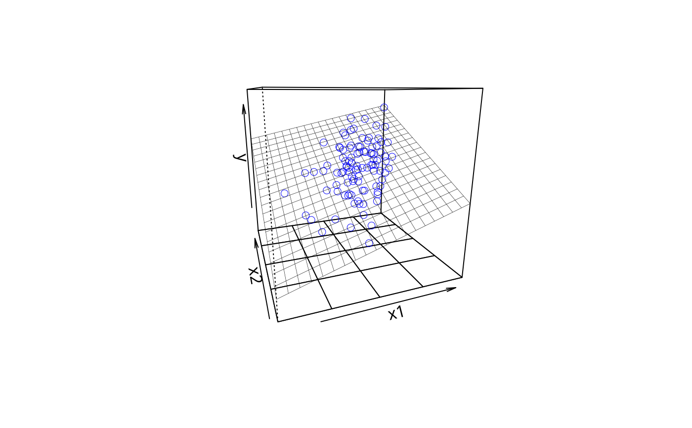
plotPlane(m3, "x1", "x2")
 m3c1 <- meanCenter(m3)
summary(m3c1)
#> These variables were mean-centered before any transformations were made on the design matrix.
#> [1] "x1c" "x2c"
#> The centers and scale factors were
#> x1c x2c
#> mean 102.2981 200.3176
#> scale 1.0000 1.0000
#> The summary statistics of the variables in the design matrix (after centering).
#> mean std.dev.
#> y 60.148 15.1175
#> x1c 0.000 18.6811
#> x2c 0.000 31.6105
#> x3some 0.250 0.4352
#> x3much 0.250 0.4352
#> x3total 0.250 0.4352
#> x1c:x2c 227.762 530.1327
#>
#> The following results were produced from:
#> meanCenter.default(model = m3)
#>
#> Call:
#> lm(formula = y ~ x1c * x2c + x3, data = stddat)
#>
#> Residuals:
#> Min 1Q Median 3Q Max
#> -26.834 -8.511 1.840 8.121 26.512
#>
#> Coefficients:
#> Estimate Std. Error t value Pr(>|t|)
#> (Intercept) 61.3923191 2.5407152 24.163 < 2e-16 ***
#> x1c 0.2141069 0.0725932 2.949 0.00403 **
#> x2c 0.2375320 0.0415086 5.722 1.27e-07 ***
#> x3some -1.6482791 3.3781023 -0.488 0.62675
#> x3much -2.0048704 3.4617949 -0.579 0.56389
#> x3total -0.9791906 3.4663022 -0.282 0.77820
#> x1c:x2c -0.0003786 0.0023661 -0.160 0.87322
#> ---
#> Signif. codes: 0 ‘***’ 0.001 ‘**’ 0.01 ‘*’ 0.05 ‘.’ 0.1 ‘ ’ 1
#>
#> Residual standard error: 11.85 on 93 degrees of freedom
#> Multiple R-squared: 0.4227, Adjusted R-squared: 0.3854
#> F-statistic: 11.35 on 6 and 93 DF, p-value: 1.754e-09
#>
## Not exactly the same as a "standardized" regression because the
## interactive variables are centered in the model frame,
## and the term "x1:x2" is never centered again.
m3c2 <- meanCenter(m3, centerDV = TRUE,
centerOnlyInteractors = FALSE, standardize = TRUE)
summary(m3c2)
#> These variables were mean-centered before any transformations were made on the design matrix.
#> [1] "ycs" "x1cs" "x2cs"
#> The centers and scale factors were
#> ycs x1cs x2cs
#> mean 60.14800 102.29814 200.31763
#> scale 15.11747 18.68108 31.61046
#> The summary statistics of the variables in the design matrix (after centering).
#> mean std.dev.
#> ycs 0.000000 1.0000000
#> x1cs 0.000000 1.0000000
#> x2cs 0.000000 1.0000000
#> x3some 0.250000 0.4351941
#> x3much 0.250000 0.4351941
#> x3total 0.250000 0.4351941
#> x1cs:x2cs 0.385699 0.8977427
#>
#> The following results were produced from:
#> meanCenter.default(model = m3, centerOnlyInteractors = FALSE,
#> centerDV = TRUE, standardize = TRUE)
#>
#> Call:
#> lm(formula = ycs ~ x1cs * x2cs + x3, data = stddat)
#>
#> Residuals:
#> Min 1Q Median 3Q Max
#> -1.7750 -0.5630 0.1217 0.5372 1.7537
#>
#> Coefficients:
#> Estimate Std. Error t value Pr(>|t|)
#> (Intercept) 0.08231 0.16806 0.490 0.62546
#> x1cs 0.26458 0.08971 2.949 0.00403 **
#> x2cs 0.49668 0.08679 5.722 1.27e-07 ***
#> x3some -0.10903 0.22346 -0.488 0.62675
#> x3much -0.13262 0.22899 -0.579 0.56389
#> x3total -0.06477 0.22929 -0.282 0.77820
#> x1cs:x2cs -0.01479 0.09242 -0.160 0.87322
#> ---
#> Signif. codes: 0 ‘***’ 0.001 ‘**’ 0.01 ‘*’ 0.05 ‘.’ 0.1 ‘ ’ 1
#>
#> Residual standard error: 0.7839 on 93 degrees of freedom
#> Multiple R-squared: 0.4227, Adjusted R-squared: 0.3854
#> F-statistic: 11.35 on 6 and 93 DF, p-value: 1.754e-09
#>
m3st <- standardize(m3)
summary(m3st)
#> All variables in the model matrix and the dependent variable
#> were centered. The centered variables have the letter "s" appended to their
#> non-centered counterparts, even constructed
#> variables like `x1:x2` and poly(x1,2). We agree, that's probably
#> ill-advised, but you asked for it by running standardize().
#>
#> The rockchalk function meanCenter is a smarter option, probably.
#>
#> The summary statistics of the variables in the design matrix.
#> mean std.dev.
#> ys 0 1
#> x1s 0 1
#> x2s 0 1
#> x3somes 0 1
#> x3muchs 0 1
#> x3totals 0 1
#> `x1:x2s` 0 1
#>
#> Call:
#> lm(formula = ys ~ -1 + x1s + x2s + x3somes + x3muchs + x3totals +
#> `x1:x2s`, data = stddat)
#>
#> Residuals:
#> Min 1Q Median 3Q Max
#> -1.7750 -0.5630 0.1217 0.5372 1.7537
#>
#> Coefficients:
#> Estimate Std. Error t value Pr(>|t|)
#> x1s 0.35830 0.57380 0.624 0.534
#> x2s 0.57766 0.52181 1.107 0.271
#> x3somes -0.04745 0.09673 -0.491 0.625
#> x3muchs -0.05772 0.09912 -0.582 0.562
#> x3totals -0.02819 0.09925 -0.284 0.777
#> `x1:x2s` -0.14571 0.90575 -0.161 0.873
#>
#> Residual standard error: 0.7798 on 94 degrees of freedom
#> Multiple R-squared: 0.4227, Adjusted R-squared: 0.3858
#> F-statistic: 11.47 on 6 and 94 DF, p-value: 1.36e-09
#>
## Make a bigger dataset to see effects better
N <- 500
dat <- genCorrelatedData(N = N, means = c(200,200), sds = c(60,30),
rho = 0.2, stde = 10)
dat$x3 <- rnorm(100, m = 40, s = 4)
dat$x3 <- gl(4, 25, labels = c("none", "some", "much", "total"))
dat$y2 <- with(dat,
0.4 - 0.15 * x1 + 0.04 * x1^2 -
drop(contrasts(dat$x3)[dat$x3, ] %*% c(-1.9, 0, 5.1)) +
1000* rnorm(nrow(dat)))
dat$y2 <- drop(dat$y2)
m4literal <- lm(y2 ~ x1 + I(x1*x1) + x2 + x3, data = dat)
summary(m4literal)
#>
#> Call:
#> lm(formula = y2 ~ x1 + I(x1 * x1) + x2 + x3, data = dat)
#>
#> Residuals:
#> Min 1Q Median 3Q Max
#> -2644.2 -721.1 -14.8 596.9 3287.6
#>
#> Coefficients:
#> Estimate Std. Error t value Pr(>|t|)
#> (Intercept) 9.412e+02 4.318e+02 2.180 0.02976 *
#> x1 -8.940e+00 3.302e+00 -2.707 0.00702 **
#> I(x1 * x1) 6.270e-02 7.955e-03 7.882 2.09e-14 ***
#> x2 -1.080e+00 1.527e+00 -0.707 0.47974
#> x3some -1.120e+02 1.243e+02 -0.901 0.36781
#> x3much 5.929e+01 1.244e+02 0.477 0.63382
#> x3total 2.130e+01 1.242e+02 0.171 0.86396
#> ---
#> Signif. codes: 0 ‘***’ 0.001 ‘**’ 0.01 ‘*’ 0.05 ‘.’ 0.1 ‘ ’ 1
#>
#> Residual standard error: 979.8 on 493 degrees of freedom
#> Multiple R-squared: 0.5293, Adjusted R-squared: 0.5235
#> F-statistic: 92.39 on 6 and 493 DF, p-value: < 2.2e-16
#>
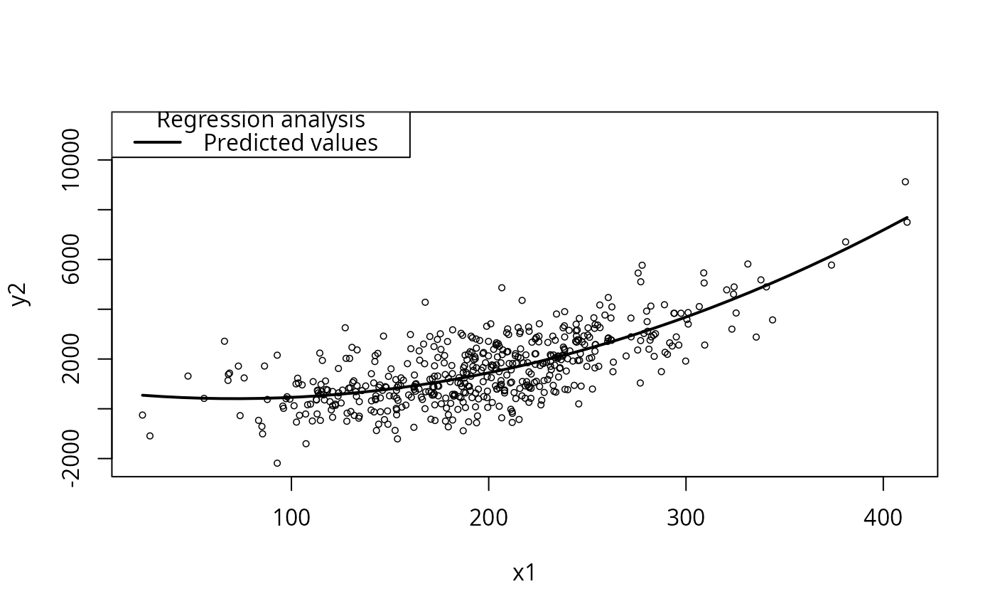
plotCurves(m4literal, plotx="x1")
m3c1 <- meanCenter(m3)
summary(m3c1)
#> These variables were mean-centered before any transformations were made on the design matrix.
#> [1] "x1c" "x2c"
#> The centers and scale factors were
#> x1c x2c
#> mean 102.2981 200.3176
#> scale 1.0000 1.0000
#> The summary statistics of the variables in the design matrix (after centering).
#> mean std.dev.
#> y 60.148 15.1175
#> x1c 0.000 18.6811
#> x2c 0.000 31.6105
#> x3some 0.250 0.4352
#> x3much 0.250 0.4352
#> x3total 0.250 0.4352
#> x1c:x2c 227.762 530.1327
#>
#> The following results were produced from:
#> meanCenter.default(model = m3)
#>
#> Call:
#> lm(formula = y ~ x1c * x2c + x3, data = stddat)
#>
#> Residuals:
#> Min 1Q Median 3Q Max
#> -26.834 -8.511 1.840 8.121 26.512
#>
#> Coefficients:
#> Estimate Std. Error t value Pr(>|t|)
#> (Intercept) 61.3923191 2.5407152 24.163 < 2e-16 ***
#> x1c 0.2141069 0.0725932 2.949 0.00403 **
#> x2c 0.2375320 0.0415086 5.722 1.27e-07 ***
#> x3some -1.6482791 3.3781023 -0.488 0.62675
#> x3much -2.0048704 3.4617949 -0.579 0.56389
#> x3total -0.9791906 3.4663022 -0.282 0.77820
#> x1c:x2c -0.0003786 0.0023661 -0.160 0.87322
#> ---
#> Signif. codes: 0 ‘***’ 0.001 ‘**’ 0.01 ‘*’ 0.05 ‘.’ 0.1 ‘ ’ 1
#>
#> Residual standard error: 11.85 on 93 degrees of freedom
#> Multiple R-squared: 0.4227, Adjusted R-squared: 0.3854
#> F-statistic: 11.35 on 6 and 93 DF, p-value: 1.754e-09
#>
## Not exactly the same as a "standardized" regression because the
## interactive variables are centered in the model frame,
## and the term "x1:x2" is never centered again.
m3c2 <- meanCenter(m3, centerDV = TRUE,
centerOnlyInteractors = FALSE, standardize = TRUE)
summary(m3c2)
#> These variables were mean-centered before any transformations were made on the design matrix.
#> [1] "ycs" "x1cs" "x2cs"
#> The centers and scale factors were
#> ycs x1cs x2cs
#> mean 60.14800 102.29814 200.31763
#> scale 15.11747 18.68108 31.61046
#> The summary statistics of the variables in the design matrix (after centering).
#> mean std.dev.
#> ycs 0.000000 1.0000000
#> x1cs 0.000000 1.0000000
#> x2cs 0.000000 1.0000000
#> x3some 0.250000 0.4351941
#> x3much 0.250000 0.4351941
#> x3total 0.250000 0.4351941
#> x1cs:x2cs 0.385699 0.8977427
#>
#> The following results were produced from:
#> meanCenter.default(model = m3, centerOnlyInteractors = FALSE,
#> centerDV = TRUE, standardize = TRUE)
#>
#> Call:
#> lm(formula = ycs ~ x1cs * x2cs + x3, data = stddat)
#>
#> Residuals:
#> Min 1Q Median 3Q Max
#> -1.7750 -0.5630 0.1217 0.5372 1.7537
#>
#> Coefficients:
#> Estimate Std. Error t value Pr(>|t|)
#> (Intercept) 0.08231 0.16806 0.490 0.62546
#> x1cs 0.26458 0.08971 2.949 0.00403 **
#> x2cs 0.49668 0.08679 5.722 1.27e-07 ***
#> x3some -0.10903 0.22346 -0.488 0.62675
#> x3much -0.13262 0.22899 -0.579 0.56389
#> x3total -0.06477 0.22929 -0.282 0.77820
#> x1cs:x2cs -0.01479 0.09242 -0.160 0.87322
#> ---
#> Signif. codes: 0 ‘***’ 0.001 ‘**’ 0.01 ‘*’ 0.05 ‘.’ 0.1 ‘ ’ 1
#>
#> Residual standard error: 0.7839 on 93 degrees of freedom
#> Multiple R-squared: 0.4227, Adjusted R-squared: 0.3854
#> F-statistic: 11.35 on 6 and 93 DF, p-value: 1.754e-09
#>
m3st <- standardize(m3)
summary(m3st)
#> All variables in the model matrix and the dependent variable
#> were centered. The centered variables have the letter "s" appended to their
#> non-centered counterparts, even constructed
#> variables like `x1:x2` and poly(x1,2). We agree, that's probably
#> ill-advised, but you asked for it by running standardize().
#>
#> The rockchalk function meanCenter is a smarter option, probably.
#>
#> The summary statistics of the variables in the design matrix.
#> mean std.dev.
#> ys 0 1
#> x1s 0 1
#> x2s 0 1
#> x3somes 0 1
#> x3muchs 0 1
#> x3totals 0 1
#> `x1:x2s` 0 1
#>
#> Call:
#> lm(formula = ys ~ -1 + x1s + x2s + x3somes + x3muchs + x3totals +
#> `x1:x2s`, data = stddat)
#>
#> Residuals:
#> Min 1Q Median 3Q Max
#> -1.7750 -0.5630 0.1217 0.5372 1.7537
#>
#> Coefficients:
#> Estimate Std. Error t value Pr(>|t|)
#> x1s 0.35830 0.57380 0.624 0.534
#> x2s 0.57766 0.52181 1.107 0.271
#> x3somes -0.04745 0.09673 -0.491 0.625
#> x3muchs -0.05772 0.09912 -0.582 0.562
#> x3totals -0.02819 0.09925 -0.284 0.777
#> `x1:x2s` -0.14571 0.90575 -0.161 0.873
#>
#> Residual standard error: 0.7798 on 94 degrees of freedom
#> Multiple R-squared: 0.4227, Adjusted R-squared: 0.3858
#> F-statistic: 11.47 on 6 and 94 DF, p-value: 1.36e-09
#>
## Make a bigger dataset to see effects better
N <- 500
dat <- genCorrelatedData(N = N, means = c(200,200), sds = c(60,30),
rho = 0.2, stde = 10)
dat$x3 <- rnorm(100, m = 40, s = 4)
dat$x3 <- gl(4, 25, labels = c("none", "some", "much", "total"))
dat$y2 <- with(dat,
0.4 - 0.15 * x1 + 0.04 * x1^2 -
drop(contrasts(dat$x3)[dat$x3, ] %*% c(-1.9, 0, 5.1)) +
1000* rnorm(nrow(dat)))
dat$y2 <- drop(dat$y2)
m4literal <- lm(y2 ~ x1 + I(x1*x1) + x2 + x3, data = dat)
summary(m4literal)
#>
#> Call:
#> lm(formula = y2 ~ x1 + I(x1 * x1) + x2 + x3, data = dat)
#>
#> Residuals:
#> Min 1Q Median 3Q Max
#> -2644.2 -721.1 -14.8 596.9 3287.6
#>
#> Coefficients:
#> Estimate Std. Error t value Pr(>|t|)
#> (Intercept) 9.412e+02 4.318e+02 2.180 0.02976 *
#> x1 -8.940e+00 3.302e+00 -2.707 0.00702 **
#> I(x1 * x1) 6.270e-02 7.955e-03 7.882 2.09e-14 ***
#> x2 -1.080e+00 1.527e+00 -0.707 0.47974
#> x3some -1.120e+02 1.243e+02 -0.901 0.36781
#> x3much 5.929e+01 1.244e+02 0.477 0.63382
#> x3total 2.130e+01 1.242e+02 0.171 0.86396
#> ---
#> Signif. codes: 0 ‘***’ 0.001 ‘**’ 0.01 ‘*’ 0.05 ‘.’ 0.1 ‘ ’ 1
#>
#> Residual standard error: 979.8 on 493 degrees of freedom
#> Multiple R-squared: 0.5293, Adjusted R-squared: 0.5235
#> F-statistic: 92.39 on 6 and 493 DF, p-value: < 2.2e-16
#>
plotCurves(m4literal, plotx="x1")
 ## Superficially, there is multicollinearity (omit the intercept)
cor(model.matrix(m4literal)[ -1 , -1 ])
#> x1 I(x1 * x1) x2 x3some x3much
#> x1 1.000000000 0.97484776 0.200596889 0.055596995 -0.03568623
#> I(x1 * x1) 0.974847755 1.00000000 0.193916204 0.044145556 -0.03810690
#> x2 0.200596889 0.19391620 1.000000000 0.004033362 0.04724582
#> x3some 0.055596995 0.04414556 0.004033362 1.000000000 -0.33422460
#> x3much -0.035686229 -0.03810690 0.047245820 -0.334224599 1.00000000
#> x3total 0.002703986 0.01114203 0.029117095 -0.334224599 -0.33422460
#> x3total
#> x1 0.002703986
#> I(x1 * x1) 0.011142031
#> x2 0.029117095
#> x3some -0.334224599
#> x3much -0.334224599
#> x3total 1.000000000
m4literalmc <- meanCenter(m4literal, terms = "x1")
summary(m4literalmc)
#> These variables were mean-centered before any transformations were made on the design matrix.
#> [1] "x1c"
#> The centers and scale factors were
#> x1c
#> mean 196.3668
#> scale 1.0000
#> The summary statistics of the variables in the design matrix (after centering).
#> mean std.dev.
#> y2 1603.279 1419.422
#> x1c 0.000 59.776
#> I(x1c * x1c) 3566.035 5562.310
#> x2 199.914 29.439
#> x3some 0.250 0.433
#> x3much 0.250 0.433
#> x3total 0.250 0.433
#>
#> The following results were produced from:
#> meanCenter.default(model = m4literal, terms = "x1")
#>
#> Call:
#> lm(formula = y2 ~ x1c + I(x1c * x1c) + x2 + x3, data = stddat)
#>
#> Residuals:
#> Min 1Q Median 3Q Max
#> -2644.2 -721.1 -14.8 596.9 3287.6
#>
#> Coefficients:
#> Estimate Std. Error t value Pr(>|t|)
#> (Intercept) 1.603e+03 3.134e+02 5.117 4.47e-07 ***
#> x1c 1.568e+01 7.560e-01 20.747 < 2e-16 ***
#> I(x1c * x1c) 6.270e-02 7.955e-03 7.882 2.09e-14 ***
#> x2 -1.080e+00 1.527e+00 -0.707 0.480
#> x3some -1.120e+02 1.243e+02 -0.901 0.368
#> x3much 5.929e+01 1.244e+02 0.477 0.634
#> x3total 2.130e+01 1.242e+02 0.171 0.864
#> ---
#> Signif. codes: 0 ‘***’ 0.001 ‘**’ 0.01 ‘*’ 0.05 ‘.’ 0.1 ‘ ’ 1
#>
#> Residual standard error: 979.8 on 493 degrees of freedom
#> Multiple R-squared: 0.5293, Adjusted R-squared: 0.5235
#> F-statistic: 92.39 on 6 and 493 DF, p-value: < 2.2e-16
#>
m4literalmcs <- meanCenter(m4literal, terms = "x1", standardize = TRUE)
summary(m4literalmcs)
#> These variables were mean-centered before any transformations were made on the design matrix.
#> [1] "x1cs"
#> The centers and scale factors were
#> x1cs
#> mean 196.3668
#> scale 59.7761
#> The summary statistics of the variables in the design matrix (after centering).
#> mean std.dev.
#> y2 1603.2794 1419.4217
#> x1cs 0.0000 1.0000
#> I(x1cs * x1cs) 0.9980 1.5567
#> x2 199.9144 29.4390
#> x3some 0.2500 0.4334
#> x3much 0.2500 0.4334
#> x3total 0.2500 0.4334
#>
#> The following results were produced from:
#> meanCenter.default(model = m4literal, standardize = TRUE, terms = "x1")
#>
#> Call:
#> lm(formula = y2 ~ x1cs + I(x1cs * x1cs) + x2 + x3, data = stddat)
#>
#> Residuals:
#> Min 1Q Median 3Q Max
#> -2644.2 -721.1 -14.8 596.9 3287.6
#>
#> Coefficients:
#> Estimate Std. Error t value Pr(>|t|)
#> (Intercept) 1603.421 313.381 5.117 4.47e-07 ***
#> x1cs 937.573 45.190 20.747 < 2e-16 ***
#> I(x1cs * x1cs) 224.038 28.425 7.882 2.09e-14 ***
#> x2 -1.080 1.527 -0.707 0.480
#> x3some -112.038 124.292 -0.901 0.368
#> x3much 59.289 124.387 0.477 0.634
#> x3total 21.296 124.232 0.171 0.864
#> ---
#> Signif. codes: 0 ‘***’ 0.001 ‘**’ 0.01 ‘*’ 0.05 ‘.’ 0.1 ‘ ’ 1
#>
#> Residual standard error: 979.8 on 493 degrees of freedom
#> Multiple R-squared: 0.5293, Adjusted R-squared: 0.5235
#> F-statistic: 92.39 on 6 and 493 DF, p-value: < 2.2e-16
#>
m4 <- lm(y2 ~ poly(x1, 2, raw = TRUE) + x2 + x3, data = dat)
summary(m4)
#>
#> Call:
#> lm(formula = y2 ~ poly(x1, 2, raw = TRUE) + x2 + x3, data = dat)
#>
#> Residuals:
#> Min 1Q Median 3Q Max
#> -2644.2 -721.1 -14.8 596.9 3287.6
#>
#> Coefficients:
#> Estimate Std. Error t value Pr(>|t|)
#> (Intercept) 9.412e+02 4.318e+02 2.180 0.02976 *
#> poly(x1, 2, raw = TRUE)1 -8.940e+00 3.302e+00 -2.707 0.00702 **
#> poly(x1, 2, raw = TRUE)2 6.270e-02 7.955e-03 7.882 2.09e-14 ***
#> x2 -1.080e+00 1.527e+00 -0.707 0.47974
#> x3some -1.120e+02 1.243e+02 -0.901 0.36781
#> x3much 5.929e+01 1.244e+02 0.477 0.63382
#> x3total 2.130e+01 1.242e+02 0.171 0.86396
#> ---
#> Signif. codes: 0 ‘***’ 0.001 ‘**’ 0.01 ‘*’ 0.05 ‘.’ 0.1 ‘ ’ 1
#>
#> Residual standard error: 979.8 on 493 degrees of freedom
#> Multiple R-squared: 0.5293, Adjusted R-squared: 0.5235
#> F-statistic: 92.39 on 6 and 493 DF, p-value: < 2.2e-16
#>
plotCurves(m4, plotx="x1")
m4mc1 <- meanCenter(m4, terms = "x1")
summary(m4mc1)
#> These variables were mean-centered before any transformations were made on the design matrix.
#> [1] "x1c"
#> The centers and scale factors were
#> x1c
#> mean 196.3668
#> scale 1.0000
#> The summary statistics of the variables in the design matrix (after centering).
#> mean std.dev.
#> y2 1603.279 1419.422
#> poly(x1c, 2, raw = TRUE)1 0.000 59.776
#> poly(x1c, 2, raw = TRUE)2 3566.035 5562.310
#> x2 199.914 29.439
#> x3some 0.250 0.433
#> x3much 0.250 0.433
#> x3total 0.250 0.433
#>
#> The following results were produced from:
#> meanCenter.default(model = m4, terms = "x1")
#>
#> Call:
#> lm(formula = y2 ~ poly(x1c, 2, raw = TRUE) + x2 + x3, data = stddat)
#>
#> Residuals:
#> Min 1Q Median 3Q Max
#> -2644.2 -721.1 -14.8 596.9 3287.6
#>
#> Coefficients:
#> Estimate Std. Error t value Pr(>|t|)
#> (Intercept) 1.603e+03 3.134e+02 5.117 4.47e-07 ***
#> poly(x1c, 2, raw = TRUE)1 1.568e+01 7.560e-01 20.747 < 2e-16 ***
#> poly(x1c, 2, raw = TRUE)2 6.270e-02 7.955e-03 7.882 2.09e-14 ***
#> x2 -1.080e+00 1.527e+00 -0.707 0.480
#> x3some -1.120e+02 1.243e+02 -0.901 0.368
#> x3much 5.929e+01 1.244e+02 0.477 0.634
#> x3total 2.130e+01 1.242e+02 0.171 0.864
#> ---
#> Signif. codes: 0 ‘***’ 0.001 ‘**’ 0.01 ‘*’ 0.05 ‘.’ 0.1 ‘ ’ 1
#>
#> Residual standard error: 979.8 on 493 degrees of freedom
#> Multiple R-squared: 0.5293, Adjusted R-squared: 0.5235
#> F-statistic: 92.39 on 6 and 493 DF, p-value: < 2.2e-16
#>
m4mc2 <- meanCenter(m4, terms = "x1", standardize = TRUE)
summary(m4mc2)
#> These variables were mean-centered before any transformations were made on the design matrix.
#> [1] "x1cs"
#> The centers and scale factors were
#> x1cs
#> mean 196.3668
#> scale 59.7761
#> The summary statistics of the variables in the design matrix (after centering).
#> mean std.dev.
#> y2 1603.2794 1419.4217
#> poly(x1cs, 2, raw = TRUE)1 0.0000 1.0000
#> poly(x1cs, 2, raw = TRUE)2 0.9980 1.5567
#> x2 199.9144 29.4390
#> x3some 0.2500 0.4334
#> x3much 0.2500 0.4334
#> x3total 0.2500 0.4334
#>
#> The following results were produced from:
#> meanCenter.default(model = m4, standardize = TRUE, terms = "x1")
#>
#> Call:
#> lm(formula = y2 ~ poly(x1cs, 2, raw = TRUE) + x2 + x3, data = stddat)
#>
#> Residuals:
#> Min 1Q Median 3Q Max
#> -2644.2 -721.1 -14.8 596.9 3287.6
#>
#> Coefficients:
#> Estimate Std. Error t value Pr(>|t|)
#> (Intercept) 1603.421 313.381 5.117 4.47e-07 ***
#> poly(x1cs, 2, raw = TRUE)1 937.573 45.190 20.747 < 2e-16 ***
#> poly(x1cs, 2, raw = TRUE)2 224.038 28.425 7.882 2.09e-14 ***
#> x2 -1.080 1.527 -0.707 0.480
#> x3some -112.038 124.292 -0.901 0.368
#> x3much 59.289 124.387 0.477 0.634
#> x3total 21.296 124.232 0.171 0.864
#> ---
#> Signif. codes: 0 ‘***’ 0.001 ‘**’ 0.01 ‘*’ 0.05 ‘.’ 0.1 ‘ ’ 1
#>
#> Residual standard error: 979.8 on 493 degrees of freedom
#> Multiple R-squared: 0.5293, Adjusted R-squared: 0.5235
#> F-statistic: 92.39 on 6 and 493 DF, p-value: < 2.2e-16
#>
m4mc3 <- meanCenter(m4, terms = "x1", centerDV = TRUE, standardize = TRUE)
summary(m4mc3)
#> These variables were mean-centered before any transformations were made on the design matrix.
#> [1] "y2cs" "x1cs"
#> The centers and scale factors were
#> y2cs x1cs
#> mean 1603.279 196.3668
#> scale 1419.422 59.7761
#> The summary statistics of the variables in the design matrix (after centering).
#> mean std.dev.
#> y2cs 0.0000 1.00000
#> poly(x1cs, 2, raw = TRUE)1 0.0000 1.00000
#> poly(x1cs, 2, raw = TRUE)2 0.9980 1.55668
#> x2 199.9144 29.43904
#> x3some 0.2500 0.43345
#> x3much 0.2500 0.43345
#> x3total 0.2500 0.43345
#>
#> The following results were produced from:
#> meanCenter.default(model = m4, centerDV = TRUE, standardize = TRUE,
#> terms = "x1")
#>
#> Call:
#> lm(formula = y2cs ~ poly(x1cs, 2, raw = TRUE) + x2 + x3, data = stddat)
#>
#> Residuals:
#> Min 1Q Median 3Q Max
#> -1.86287 -0.50805 -0.01046 0.42049 2.31616
#>
#> Coefficients:
#> Estimate Std. Error t value Pr(>|t|)
#> (Intercept) 9.973e-05 2.208e-01 0.000 1.000
#> poly(x1cs, 2, raw = TRUE)1 6.605e-01 3.184e-02 20.747 < 2e-16 ***
#> poly(x1cs, 2, raw = TRUE)2 1.578e-01 2.003e-02 7.882 2.09e-14 ***
#> x2 -7.607e-04 1.076e-03 -0.707 0.480
#> x3some -7.893e-02 8.756e-02 -0.901 0.368
#> x3much 4.177e-02 8.763e-02 0.477 0.634
#> x3total 1.500e-02 8.752e-02 0.171 0.864
#> ---
#> Signif. codes: 0 ‘***’ 0.001 ‘**’ 0.01 ‘*’ 0.05 ‘.’ 0.1 ‘ ’ 1
#>
#> Residual standard error: 0.6903 on 493 degrees of freedom
#> Multiple R-squared: 0.5293, Adjusted R-squared: 0.5235
#> F-statistic: 92.39 on 6 and 493 DF, p-value: < 2.2e-16
#>
## Superficially, there is multicollinearity (omit the intercept)
cor(model.matrix(m4literal)[ -1 , -1 ])
#> x1 I(x1 * x1) x2 x3some x3much
#> x1 1.000000000 0.97484776 0.200596889 0.055596995 -0.03568623
#> I(x1 * x1) 0.974847755 1.00000000 0.193916204 0.044145556 -0.03810690
#> x2 0.200596889 0.19391620 1.000000000 0.004033362 0.04724582
#> x3some 0.055596995 0.04414556 0.004033362 1.000000000 -0.33422460
#> x3much -0.035686229 -0.03810690 0.047245820 -0.334224599 1.00000000
#> x3total 0.002703986 0.01114203 0.029117095 -0.334224599 -0.33422460
#> x3total
#> x1 0.002703986
#> I(x1 * x1) 0.011142031
#> x2 0.029117095
#> x3some -0.334224599
#> x3much -0.334224599
#> x3total 1.000000000
m4literalmc <- meanCenter(m4literal, terms = "x1")
summary(m4literalmc)
#> These variables were mean-centered before any transformations were made on the design matrix.
#> [1] "x1c"
#> The centers and scale factors were
#> x1c
#> mean 196.3668
#> scale 1.0000
#> The summary statistics of the variables in the design matrix (after centering).
#> mean std.dev.
#> y2 1603.279 1419.422
#> x1c 0.000 59.776
#> I(x1c * x1c) 3566.035 5562.310
#> x2 199.914 29.439
#> x3some 0.250 0.433
#> x3much 0.250 0.433
#> x3total 0.250 0.433
#>
#> The following results were produced from:
#> meanCenter.default(model = m4literal, terms = "x1")
#>
#> Call:
#> lm(formula = y2 ~ x1c + I(x1c * x1c) + x2 + x3, data = stddat)
#>
#> Residuals:
#> Min 1Q Median 3Q Max
#> -2644.2 -721.1 -14.8 596.9 3287.6
#>
#> Coefficients:
#> Estimate Std. Error t value Pr(>|t|)
#> (Intercept) 1.603e+03 3.134e+02 5.117 4.47e-07 ***
#> x1c 1.568e+01 7.560e-01 20.747 < 2e-16 ***
#> I(x1c * x1c) 6.270e-02 7.955e-03 7.882 2.09e-14 ***
#> x2 -1.080e+00 1.527e+00 -0.707 0.480
#> x3some -1.120e+02 1.243e+02 -0.901 0.368
#> x3much 5.929e+01 1.244e+02 0.477 0.634
#> x3total 2.130e+01 1.242e+02 0.171 0.864
#> ---
#> Signif. codes: 0 ‘***’ 0.001 ‘**’ 0.01 ‘*’ 0.05 ‘.’ 0.1 ‘ ’ 1
#>
#> Residual standard error: 979.8 on 493 degrees of freedom
#> Multiple R-squared: 0.5293, Adjusted R-squared: 0.5235
#> F-statistic: 92.39 on 6 and 493 DF, p-value: < 2.2e-16
#>
m4literalmcs <- meanCenter(m4literal, terms = "x1", standardize = TRUE)
summary(m4literalmcs)
#> These variables were mean-centered before any transformations were made on the design matrix.
#> [1] "x1cs"
#> The centers and scale factors were
#> x1cs
#> mean 196.3668
#> scale 59.7761
#> The summary statistics of the variables in the design matrix (after centering).
#> mean std.dev.
#> y2 1603.2794 1419.4217
#> x1cs 0.0000 1.0000
#> I(x1cs * x1cs) 0.9980 1.5567
#> x2 199.9144 29.4390
#> x3some 0.2500 0.4334
#> x3much 0.2500 0.4334
#> x3total 0.2500 0.4334
#>
#> The following results were produced from:
#> meanCenter.default(model = m4literal, standardize = TRUE, terms = "x1")
#>
#> Call:
#> lm(formula = y2 ~ x1cs + I(x1cs * x1cs) + x2 + x3, data = stddat)
#>
#> Residuals:
#> Min 1Q Median 3Q Max
#> -2644.2 -721.1 -14.8 596.9 3287.6
#>
#> Coefficients:
#> Estimate Std. Error t value Pr(>|t|)
#> (Intercept) 1603.421 313.381 5.117 4.47e-07 ***
#> x1cs 937.573 45.190 20.747 < 2e-16 ***
#> I(x1cs * x1cs) 224.038 28.425 7.882 2.09e-14 ***
#> x2 -1.080 1.527 -0.707 0.480
#> x3some -112.038 124.292 -0.901 0.368
#> x3much 59.289 124.387 0.477 0.634
#> x3total 21.296 124.232 0.171 0.864
#> ---
#> Signif. codes: 0 ‘***’ 0.001 ‘**’ 0.01 ‘*’ 0.05 ‘.’ 0.1 ‘ ’ 1
#>
#> Residual standard error: 979.8 on 493 degrees of freedom
#> Multiple R-squared: 0.5293, Adjusted R-squared: 0.5235
#> F-statistic: 92.39 on 6 and 493 DF, p-value: < 2.2e-16
#>
m4 <- lm(y2 ~ poly(x1, 2, raw = TRUE) + x2 + x3, data = dat)
summary(m4)
#>
#> Call:
#> lm(formula = y2 ~ poly(x1, 2, raw = TRUE) + x2 + x3, data = dat)
#>
#> Residuals:
#> Min 1Q Median 3Q Max
#> -2644.2 -721.1 -14.8 596.9 3287.6
#>
#> Coefficients:
#> Estimate Std. Error t value Pr(>|t|)
#> (Intercept) 9.412e+02 4.318e+02 2.180 0.02976 *
#> poly(x1, 2, raw = TRUE)1 -8.940e+00 3.302e+00 -2.707 0.00702 **
#> poly(x1, 2, raw = TRUE)2 6.270e-02 7.955e-03 7.882 2.09e-14 ***
#> x2 -1.080e+00 1.527e+00 -0.707 0.47974
#> x3some -1.120e+02 1.243e+02 -0.901 0.36781
#> x3much 5.929e+01 1.244e+02 0.477 0.63382
#> x3total 2.130e+01 1.242e+02 0.171 0.86396
#> ---
#> Signif. codes: 0 ‘***’ 0.001 ‘**’ 0.01 ‘*’ 0.05 ‘.’ 0.1 ‘ ’ 1
#>
#> Residual standard error: 979.8 on 493 degrees of freedom
#> Multiple R-squared: 0.5293, Adjusted R-squared: 0.5235
#> F-statistic: 92.39 on 6 and 493 DF, p-value: < 2.2e-16
#>
plotCurves(m4, plotx="x1")
m4mc1 <- meanCenter(m4, terms = "x1")
summary(m4mc1)
#> These variables were mean-centered before any transformations were made on the design matrix.
#> [1] "x1c"
#> The centers and scale factors were
#> x1c
#> mean 196.3668
#> scale 1.0000
#> The summary statistics of the variables in the design matrix (after centering).
#> mean std.dev.
#> y2 1603.279 1419.422
#> poly(x1c, 2, raw = TRUE)1 0.000 59.776
#> poly(x1c, 2, raw = TRUE)2 3566.035 5562.310
#> x2 199.914 29.439
#> x3some 0.250 0.433
#> x3much 0.250 0.433
#> x3total 0.250 0.433
#>
#> The following results were produced from:
#> meanCenter.default(model = m4, terms = "x1")
#>
#> Call:
#> lm(formula = y2 ~ poly(x1c, 2, raw = TRUE) + x2 + x3, data = stddat)
#>
#> Residuals:
#> Min 1Q Median 3Q Max
#> -2644.2 -721.1 -14.8 596.9 3287.6
#>
#> Coefficients:
#> Estimate Std. Error t value Pr(>|t|)
#> (Intercept) 1.603e+03 3.134e+02 5.117 4.47e-07 ***
#> poly(x1c, 2, raw = TRUE)1 1.568e+01 7.560e-01 20.747 < 2e-16 ***
#> poly(x1c, 2, raw = TRUE)2 6.270e-02 7.955e-03 7.882 2.09e-14 ***
#> x2 -1.080e+00 1.527e+00 -0.707 0.480
#> x3some -1.120e+02 1.243e+02 -0.901 0.368
#> x3much 5.929e+01 1.244e+02 0.477 0.634
#> x3total 2.130e+01 1.242e+02 0.171 0.864
#> ---
#> Signif. codes: 0 ‘***’ 0.001 ‘**’ 0.01 ‘*’ 0.05 ‘.’ 0.1 ‘ ’ 1
#>
#> Residual standard error: 979.8 on 493 degrees of freedom
#> Multiple R-squared: 0.5293, Adjusted R-squared: 0.5235
#> F-statistic: 92.39 on 6 and 493 DF, p-value: < 2.2e-16
#>
m4mc2 <- meanCenter(m4, terms = "x1", standardize = TRUE)
summary(m4mc2)
#> These variables were mean-centered before any transformations were made on the design matrix.
#> [1] "x1cs"
#> The centers and scale factors were
#> x1cs
#> mean 196.3668
#> scale 59.7761
#> The summary statistics of the variables in the design matrix (after centering).
#> mean std.dev.
#> y2 1603.2794 1419.4217
#> poly(x1cs, 2, raw = TRUE)1 0.0000 1.0000
#> poly(x1cs, 2, raw = TRUE)2 0.9980 1.5567
#> x2 199.9144 29.4390
#> x3some 0.2500 0.4334
#> x3much 0.2500 0.4334
#> x3total 0.2500 0.4334
#>
#> The following results were produced from:
#> meanCenter.default(model = m4, standardize = TRUE, terms = "x1")
#>
#> Call:
#> lm(formula = y2 ~ poly(x1cs, 2, raw = TRUE) + x2 + x3, data = stddat)
#>
#> Residuals:
#> Min 1Q Median 3Q Max
#> -2644.2 -721.1 -14.8 596.9 3287.6
#>
#> Coefficients:
#> Estimate Std. Error t value Pr(>|t|)
#> (Intercept) 1603.421 313.381 5.117 4.47e-07 ***
#> poly(x1cs, 2, raw = TRUE)1 937.573 45.190 20.747 < 2e-16 ***
#> poly(x1cs, 2, raw = TRUE)2 224.038 28.425 7.882 2.09e-14 ***
#> x2 -1.080 1.527 -0.707 0.480
#> x3some -112.038 124.292 -0.901 0.368
#> x3much 59.289 124.387 0.477 0.634
#> x3total 21.296 124.232 0.171 0.864
#> ---
#> Signif. codes: 0 ‘***’ 0.001 ‘**’ 0.01 ‘*’ 0.05 ‘.’ 0.1 ‘ ’ 1
#>
#> Residual standard error: 979.8 on 493 degrees of freedom
#> Multiple R-squared: 0.5293, Adjusted R-squared: 0.5235
#> F-statistic: 92.39 on 6 and 493 DF, p-value: < 2.2e-16
#>
m4mc3 <- meanCenter(m4, terms = "x1", centerDV = TRUE, standardize = TRUE)
summary(m4mc3)
#> These variables were mean-centered before any transformations were made on the design matrix.
#> [1] "y2cs" "x1cs"
#> The centers and scale factors were
#> y2cs x1cs
#> mean 1603.279 196.3668
#> scale 1419.422 59.7761
#> The summary statistics of the variables in the design matrix (after centering).
#> mean std.dev.
#> y2cs 0.0000 1.00000
#> poly(x1cs, 2, raw = TRUE)1 0.0000 1.00000
#> poly(x1cs, 2, raw = TRUE)2 0.9980 1.55668
#> x2 199.9144 29.43904
#> x3some 0.2500 0.43345
#> x3much 0.2500 0.43345
#> x3total 0.2500 0.43345
#>
#> The following results were produced from:
#> meanCenter.default(model = m4, centerDV = TRUE, standardize = TRUE,
#> terms = "x1")
#>
#> Call:
#> lm(formula = y2cs ~ poly(x1cs, 2, raw = TRUE) + x2 + x3, data = stddat)
#>
#> Residuals:
#> Min 1Q Median 3Q Max
#> -1.86287 -0.50805 -0.01046 0.42049 2.31616
#>
#> Coefficients:
#> Estimate Std. Error t value Pr(>|t|)
#> (Intercept) 9.973e-05 2.208e-01 0.000 1.000
#> poly(x1cs, 2, raw = TRUE)1 6.605e-01 3.184e-02 20.747 < 2e-16 ***
#> poly(x1cs, 2, raw = TRUE)2 1.578e-01 2.003e-02 7.882 2.09e-14 ***
#> x2 -7.607e-04 1.076e-03 -0.707 0.480
#> x3some -7.893e-02 8.756e-02 -0.901 0.368
#> x3much 4.177e-02 8.763e-02 0.477 0.634
#> x3total 1.500e-02 8.752e-02 0.171 0.864
#> ---
#> Signif. codes: 0 ‘***’ 0.001 ‘**’ 0.01 ‘*’ 0.05 ‘.’ 0.1 ‘ ’ 1
#>
#> Residual standard error: 0.6903 on 493 degrees of freedom
#> Multiple R-squared: 0.5293, Adjusted R-squared: 0.5235
#> F-statistic: 92.39 on 6 and 493 DF, p-value: < 2.2e-16
#>