Draw a 3-D regression plot for two predictors from any linear or nonlinear lm or glm object
plotPlane.RdThis allows user to fit a regression model with many variables and then plot 2 of its predictors and the output plane for those predictors with other variables set at mean or mode (numeric or factor). This is a front-end (wrapper) for R's persp function. Persp does all of the hard work, this function reorganizes the information for the user in a more readily understood way. It intended as a convenience for students (or others) who do not want to fight their way through the details needed to use persp to plot a regression plane. The fitted model can have any number of input variables, this will display only two of them. And, at least for the moment, I insist these predictors must be numeric variables. They can be transformed in any of the usual ways, such as poly, log, and so forth.
Usage
plotPlane(
  model = NULL,
  plotx1 = NULL,
  plotx2 = NULL,
  drawArrows = FALSE,
  plotPoints = TRUE,
  npp = 20,
  x1lab,
  x2lab,
  ylab,
  x1lim,
  x2lim,
  x1floor = 5,
  x2floor = 5,
  pch = 1,
  pcol = "blue",
  plwd = 0.5,
  pcex = 1,
  llwd = 0.3,
  lcol = 1,
  llty = 1,
  acol = "red",
  alty = 4,
  alwd = 0.3,
  alength = 0.1,
  linesFrom,
  lflwd = 3,
  envir = environment(formula(model)),
  ...
)

# Default S3 method
plotPlane(
  model = NULL,
  plotx1 = NULL,
  plotx2 = NULL,
  drawArrows = FALSE,
  plotPoints = TRUE,
  npp = 20,
  x1lab,
  x2lab,
  ylab,
  x1lim,
  x2lim,
  x1floor = 5,
  x2floor = 5,
  pch = 1,
  pcol = "blue",
  plwd = 0.5,
  pcex = 1,
  llwd = 0.3,
  lcol = 1,
  llty = 1,
  acol = "red",
  alty = 4,
  alwd = 0.3,
  alength = 0.1,
  linesFrom,
  lflwd = 3,
  envir = environment(formula(model)),
  ...
)
Arguments
- model
an lm or glm fitted model object
- plotx1
name of one variable to be used on the x1 axis
- plotx2
name of one variable to be used on the x2 axis
- drawArrows
draw red arrows from prediction plane toward observed values TRUE or FALSE
- plotPoints
Should the plot include scatter of observed scores?
- npp
number of points at which to calculate prediction
- x1lab
optional label
- x2lab
optional label
- ylab
optional label
- x1lim
optional lower and upper bounds for x1, as vector like c(0,1)
- x2lim
optional lower and upper bounds for x2, as vector like c(0,1)
- x1floor
Default=5. Number of "floor" lines to be drawn for variable x1
- x2floor
Default=5. Number of "floor" lines to be drawn for variable x2
- pch
plot character, passed on to the "points" function
- pcol
color for points, col passed to "points" function
- plwd
line width, lwd passed to "points" function
- pcex
character expansion, cex passed to "points" function
- llwd
line width, lwd passed to the "lines" function
- lcol
line color, col passed to the "lines" function
- llty
line type, lty passed to the "lines" function
- acol
color for arrows, col passed to "arrows" function
- alty
arrow line type, lty passed to the "arrows" function
- alwd
arrow line width, lwd passed to the "arrows" function
- alength
arrow head length, length passed to "arrows" function
- linesFrom
object with information about "highlight" lines to be added to the 3d plane (output from plotCurves or plotSlopes)
- lflwd
line widths for linesFrom highlight lines
- envir
environment from whence to grab data
- ...
additional parameters that will go to persp
Value
The main point is the plot that is drawn, but for record keeping the return object is a list including 1) res: the transformation matrix that was created by persp 2) the call that was issued, 3) x1seq, the "plot sequence" for the x1 dimension, 4) x2seq, the "plot sequence" for the x2 dimension, 5) zplane, the values of the plane corresponding to locations x1seq and x2seq.
Details
Besides a fitted model object, plotPlane requires two additional arguments, plotx1 and plotx2. These are the names of the plotting variables. Please note, that if the term in the regression is something like poly(fish,2) or log(fish), then the argument to plotx1 should be the quoted name of the variable "fish". plotPlane will handle the work of re-organizing the information so that R's predict functions can generate the desired information. This might be thought of as a 3D version of "termplot", with a significant exception. The calculation of predicted values depends on predictors besides plotx1 and plotx2 in a different ways. The sample averages are used for numeric variables, but for factors the modal value is used.
This function creates an empty 3D drawing and then fills in the
pieces. It uses the R functions lines, points, and
arrows. To allow customization, several parameters are
introduced for the users to choose colors and such. These options
are prefixed by "l" for the lines that draw the plane, "p" for the
points, and "a" for the arrows. Of course, if plotPoints=FALSE or
drawArrows=FALSE, then these options are irrelevant.
See also
persp, scatterplot3d, regr2.plot
Author
Paul E. Johnson pauljohn@ku.edu
Examples
library(rockchalk)
set.seed(12345)
x1 <- rnorm(100)
x2 <- rnorm(100)
x3 <- rnorm(100)
x4 <- rnorm(100)
y <- rnorm(100)
y2 <- 0.03 + 0.1*x1 + 0.1*x2 + 0.25*x1*x2 + 0.4*x3 -0.1*x4 + 1*rnorm(100)
dat <- data.frame(x1,x2,x3,x4,y, y2)
rm(x1, x2, x3, x4, y, y2)
## linear ordinary regression
m1 <- lm(y ~ x1 + x2 +x3 + x4, data = dat)
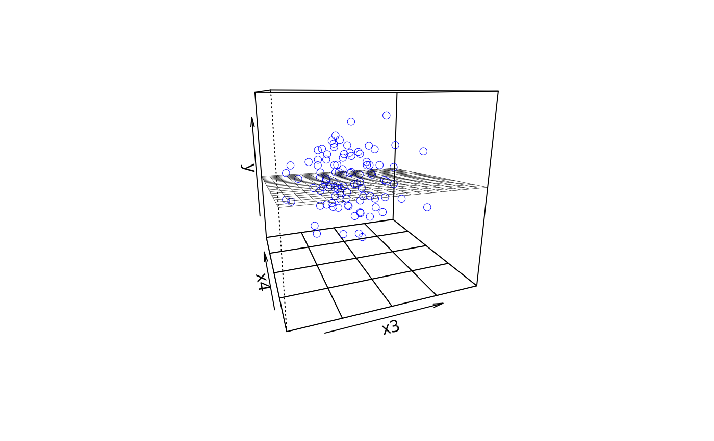
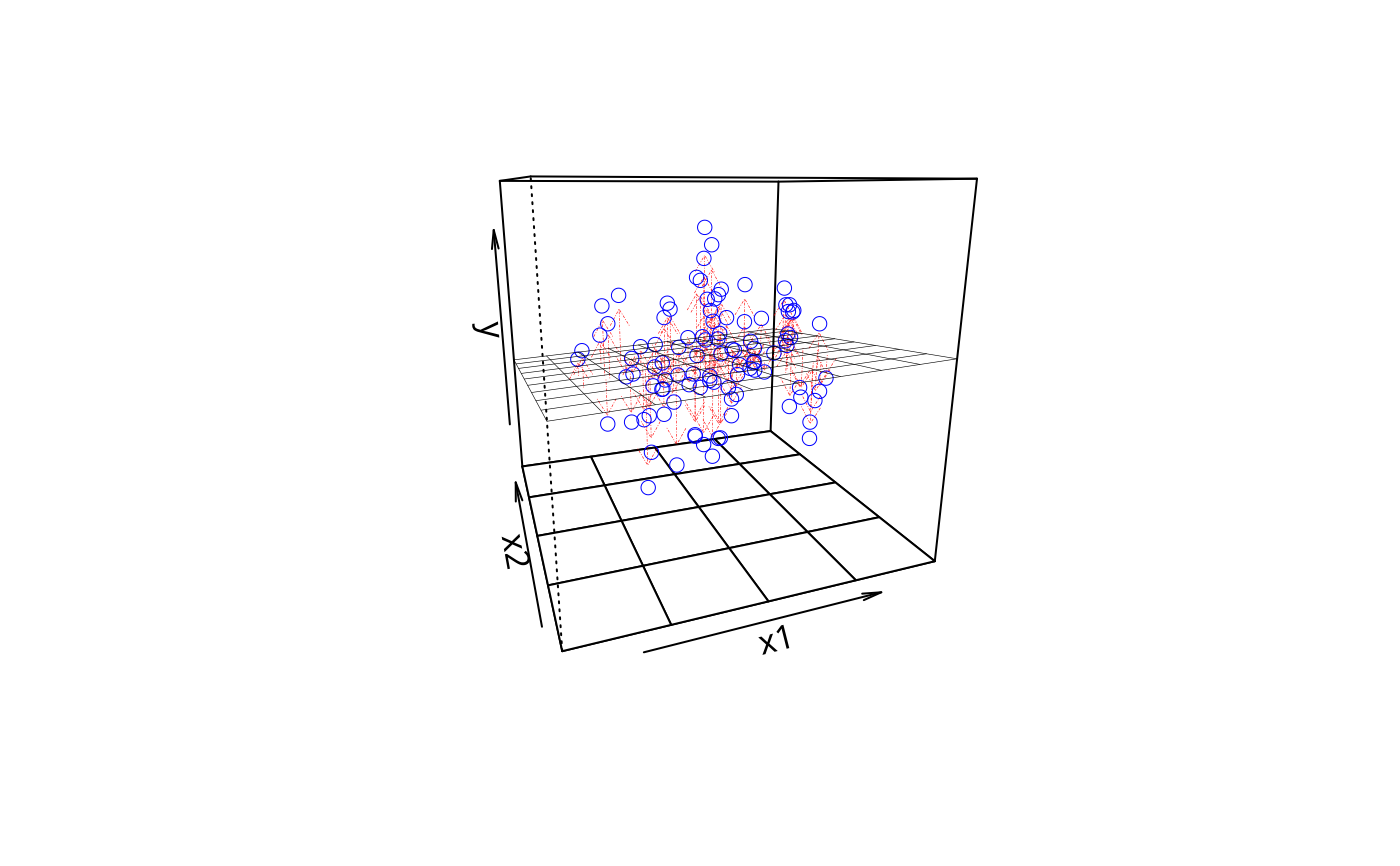
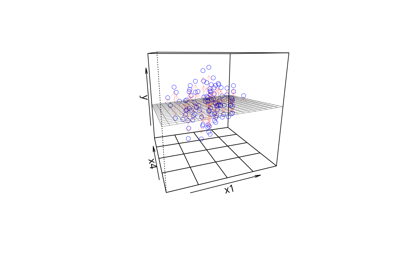
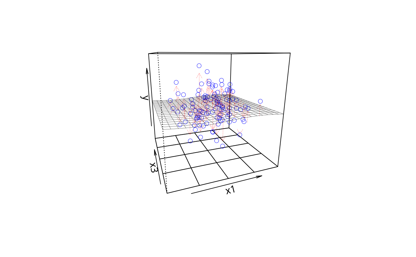
plotPlane(m1, plotx1 = "x3", plotx2 = "x4")
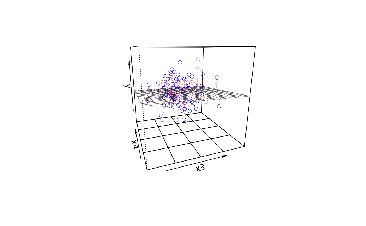
 plotPlane(m1, plotx1 = "x3", plotx2 = "x4", drawArrows = TRUE)
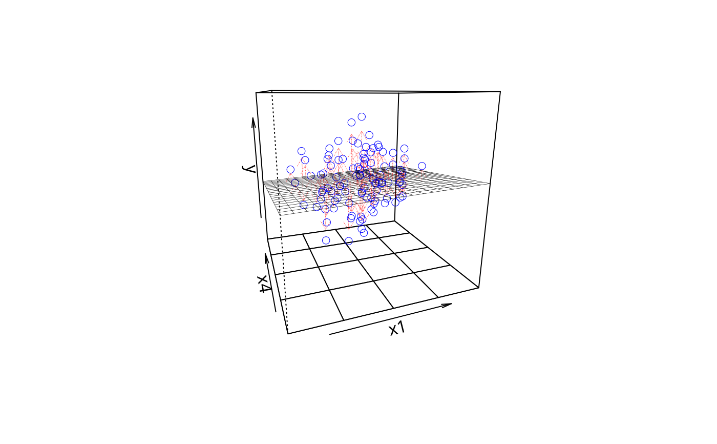
 plotPlane(m1, plotx1 = "x1", plotx2 = "x4", drawArrows = TRUE)
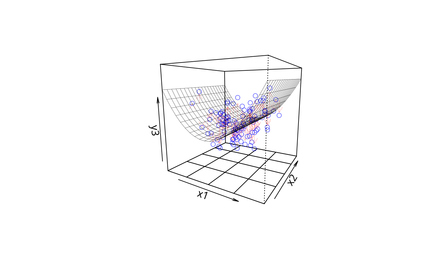
 plotPlane(m1, plotx1 = "x1", plotx2 = "x2", drawArrows = TRUE, npp = 10)
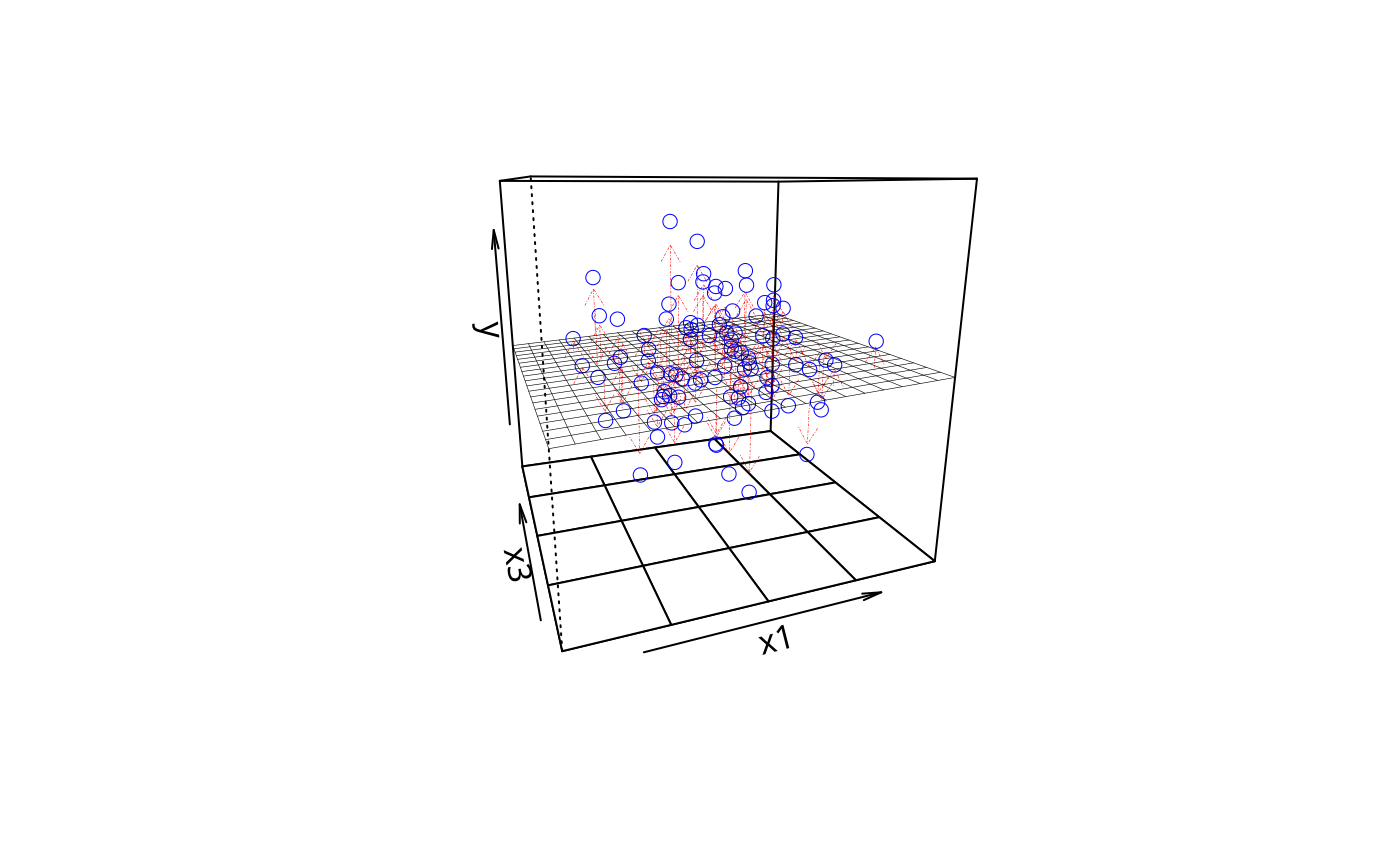
 plotPlane(m1, plotx1 = "x3", plotx2 = "x2", drawArrows = TRUE, npp = 40)
 plotPlane(m1, plotx1 = "x3", plotx2 = "x2", drawArrows = FALSE,
npp = 5, ticktype = "detailed")
plotPlane(m1, plotx1 = "x3", plotx2 = "x2", drawArrows = FALSE,
npp = 5, ticktype = "detailed")
 ## regression with interaction
m2 <- lm(y ~ x1 * x2 +x3 + x4, data = dat)
plotPlane(m2, plotx1 = "x1", plotx2 = "x2", drawArrows = TRUE)
## regression with interaction
m2 <- lm(y ~ x1 * x2 +x3 + x4, data = dat)
plotPlane(m2, plotx1 = "x1", plotx2 = "x2", drawArrows = TRUE)
 plotPlane(m2, plotx1 = "x1", plotx2 = "x4", drawArrows = TRUE)
 plotPlane(m2, plotx1 = "x1", plotx2 = "x3", drawArrows = TRUE)
 plotPlane(m2, plotx1 = "x1", plotx2 = "x2", drawArrows = TRUE,
phi = 10, theta = 30)
plotPlane(m2, plotx1 = "x1", plotx2 = "x2", drawArrows = TRUE,
phi = 10, theta = 30)
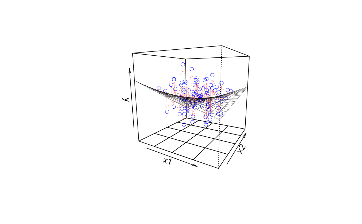 ## regression with quadratic;
## Required some fancy footwork in plotPlane, so be happy
dat$y3 <- 0 + 1 * dat$x1 + 2 * dat$x1^2 + 1 * dat$x2 +
0.4*dat$x3 + 8 * rnorm(100)
m3 <- lm(y3 ~ poly(x1,2) + x2 +x3 + x4, data = dat)
summary(m3)
#>
#> Call:
#> lm(formula = y3 ~ poly(x1, 2) + x2 + x3 + x4, data = dat)
#>
#> Residuals:
#> Min 1Q Median 3Q Max
#> -19.7909 -5.7482 0.3726 4.3458 19.1961
#>
#> Coefficients:
#> Estimate Std. Error t value Pr(>|t|)
#> (Intercept) 2.8891 0.8550 3.379 0.00106 **
#> poly(x1, 2)1 15.6691 8.4531 1.854 0.06693 .
#> poly(x1, 2)2 42.1855 8.3752 5.037 2.28e-06 ***
#> x2 0.3709 0.8463 0.438 0.66220
#> x3 -0.5161 0.9449 -0.546 0.58624
#> x4 -0.5787 0.9175 -0.631 0.52977
#> ---
#> Signif. codes: 0 ‘***’ 0.001 ‘**’ 0.01 ‘*’ 0.05 ‘.’ 0.1 ‘ ’ 1
#>
#> Residual standard error: 8.338 on 94 degrees of freedom
#> Multiple R-squared: 0.2419, Adjusted R-squared: 0.2016
#> F-statistic: 5.999 on 5 and 94 DF, p-value: 7.343e-05
#>
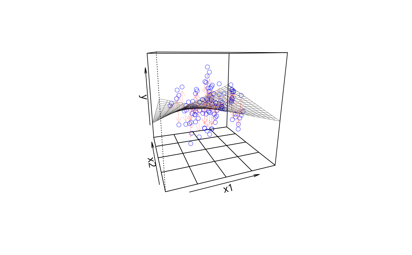
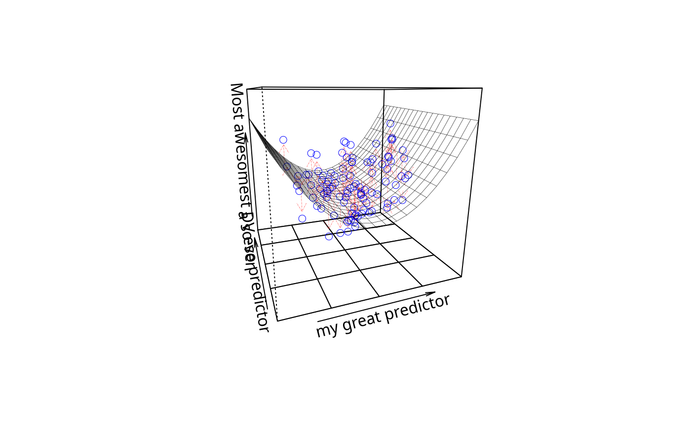
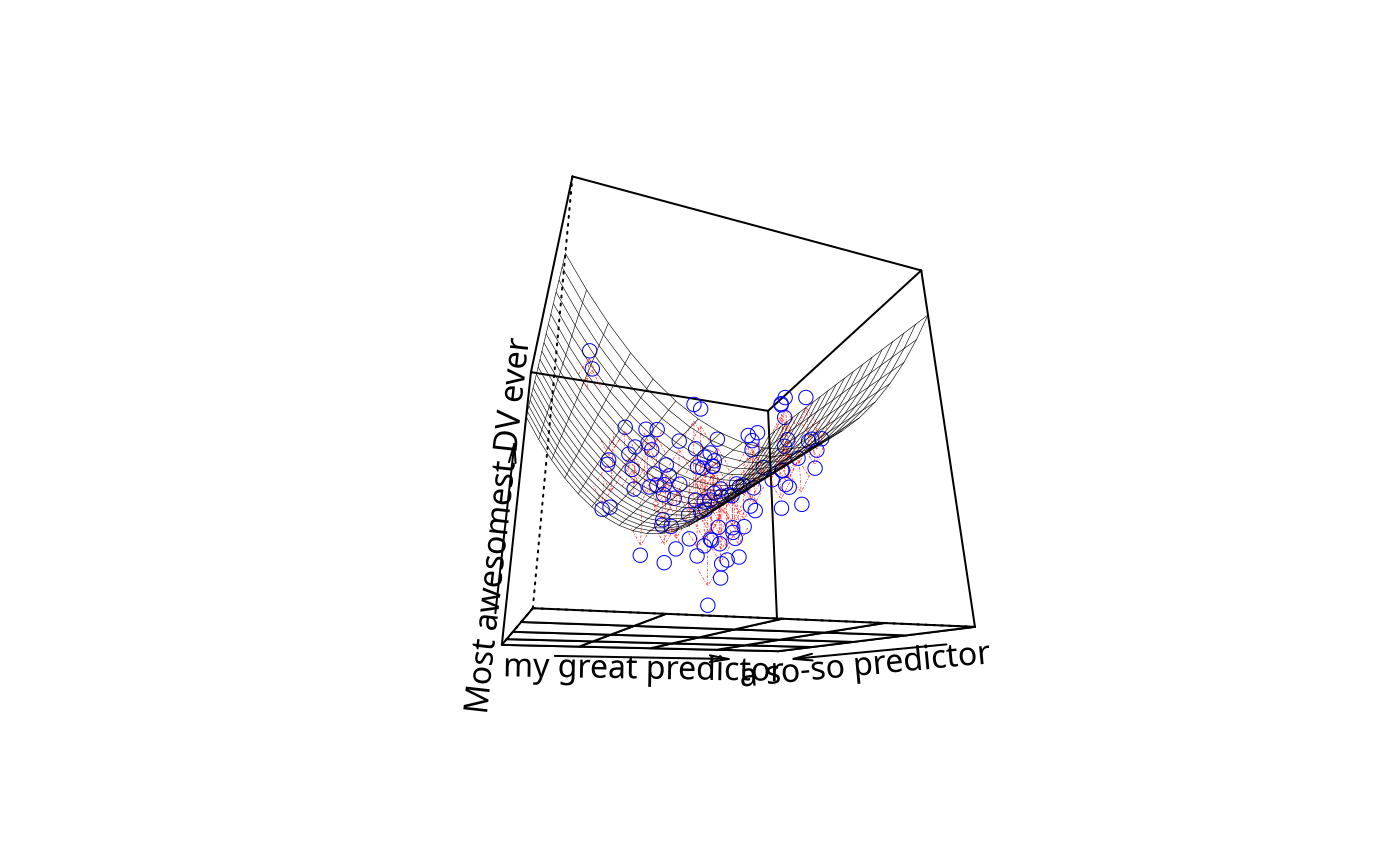
plotPlane(m3, plotx1 = "x1", plotx2 = "x2", drawArrows = TRUE,
x1lab = "my great predictor", x2lab = "a so-so predictor",
ylab = "Most awesomest DV ever")
## regression with quadratic;
## Required some fancy footwork in plotPlane, so be happy
dat$y3 <- 0 + 1 * dat$x1 + 2 * dat$x1^2 + 1 * dat$x2 +
0.4*dat$x3 + 8 * rnorm(100)
m3 <- lm(y3 ~ poly(x1,2) + x2 +x3 + x4, data = dat)
summary(m3)
#>
#> Call:
#> lm(formula = y3 ~ poly(x1, 2) + x2 + x3 + x4, data = dat)
#>
#> Residuals:
#> Min 1Q Median 3Q Max
#> -19.7909 -5.7482 0.3726 4.3458 19.1961
#>
#> Coefficients:
#> Estimate Std. Error t value Pr(>|t|)
#> (Intercept) 2.8891 0.8550 3.379 0.00106 **
#> poly(x1, 2)1 15.6691 8.4531 1.854 0.06693 .
#> poly(x1, 2)2 42.1855 8.3752 5.037 2.28e-06 ***
#> x2 0.3709 0.8463 0.438 0.66220
#> x3 -0.5161 0.9449 -0.546 0.58624
#> x4 -0.5787 0.9175 -0.631 0.52977
#> ---
#> Signif. codes: 0 ‘***’ 0.001 ‘**’ 0.01 ‘*’ 0.05 ‘.’ 0.1 ‘ ’ 1
#>
#> Residual standard error: 8.338 on 94 degrees of freedom
#> Multiple R-squared: 0.2419, Adjusted R-squared: 0.2016
#> F-statistic: 5.999 on 5 and 94 DF, p-value: 7.343e-05
#>
plotPlane(m3, plotx1 = "x1", plotx2 = "x2", drawArrows = TRUE,
x1lab = "my great predictor", x2lab = "a so-so predictor",
ylab = "Most awesomest DV ever")
 plotPlane(m3, plotx1 = "x1", plotx2 = "x2", drawArrows = TRUE,
x1lab = "my great predictor", x2lab = "a so-so predictor",
ylab = "Most awesomest DV ever", phi = -20)
plotPlane(m3, plotx1 = "x1", plotx2 = "x2", drawArrows = TRUE,
x1lab = "my great predictor", x2lab = "a so-so predictor",
ylab = "Most awesomest DV ever", phi = -20)
 plotPlane(m3, plotx1 = "x1", plotx2 = "x2", drawArrows = TRUE,
phi = 10, theta = 30)
plotPlane(m3, plotx1 = "x1", plotx2 = "x2", drawArrows = TRUE,
phi = 10, theta = 30)
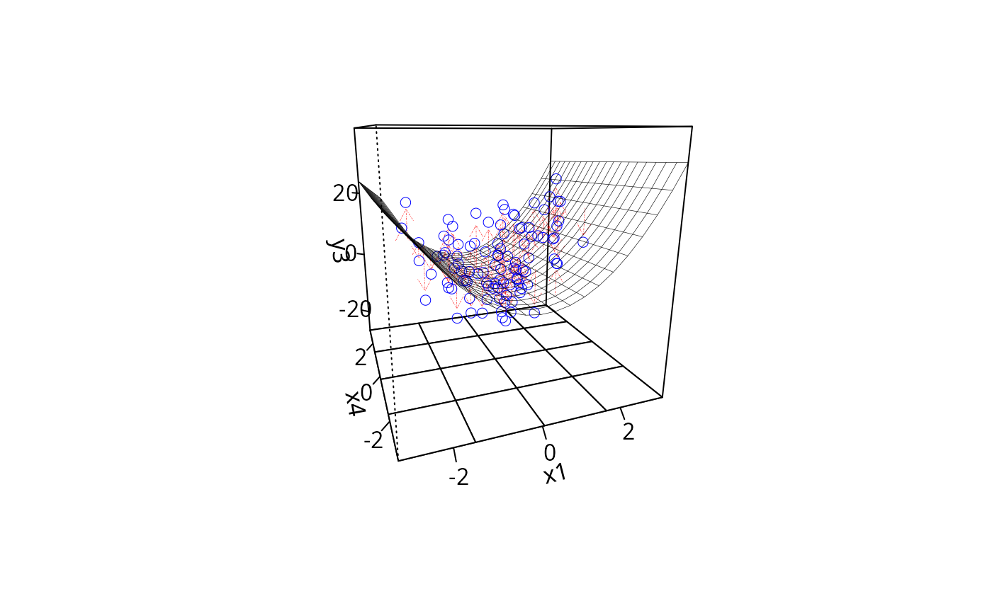
 plotPlane(m3, plotx1 = "x1", plotx2 = "x4", drawArrows = TRUE,
ticktype = "detailed")
plotPlane(m3, plotx1 = "x1", plotx2 = "x4", drawArrows = TRUE,
ticktype = "detailed")
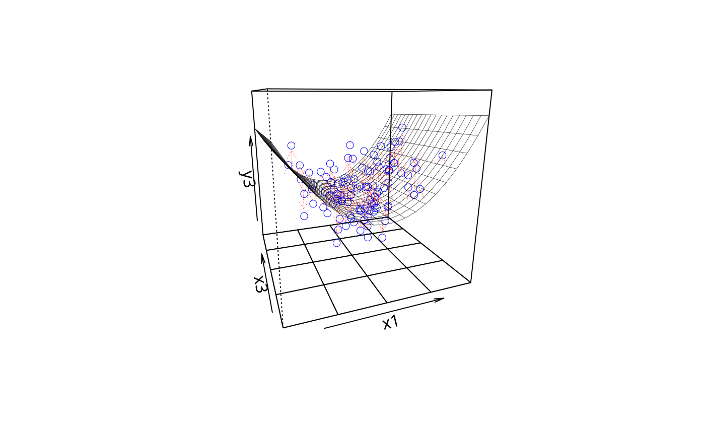
 plotPlane(m3, plotx1 = "x1", plotx2 = "x3", drawArrows = TRUE)
 plotPlane(m3, plotx1 = "x1", plotx2 = "x2", drawArrows = TRUE,
phi = 10, theta = 30)
plotPlane(m3, plotx1 = "x1", plotx2 = "x2", drawArrows = TRUE,
phi = 10, theta = 30)
 m4 <- lm(y ~ sin(x1) + x2*x3 +x3 + x4, data = dat)
summary(m4)
#>
#> Call:
#> lm(formula = y ~ sin(x1) + x2 * x3 + x3 + x4, data = dat)
#>
#> Residuals:
#> Min 1Q Median 3Q Max
#> -2.08648 -0.59177 0.03107 0.58728 2.10103
#>
#> Coefficients:
#> Estimate Std. Error t value Pr(>|t|)
#> (Intercept) -0.01732 0.09240 -0.187 0.852
#> sin(x1) 0.07440 0.12927 0.576 0.566
#> x2 -0.12962 0.08921 -1.453 0.150
#> x3 -0.02928 0.10020 -0.292 0.771
#> x4 -0.10424 0.09689 -1.076 0.285
#> x2:x3 0.11490 0.08249 1.393 0.167
#>
#> Residual standard error: 0.8819 on 94 degrees of freedom
#> Multiple R-squared: 0.05949, Adjusted R-squared: 0.009458
#> F-statistic: 1.189 on 5 and 94 DF, p-value: 0.3205
#>
plotPlane(m4, plotx1 = "x1", plotx2 = "x2", drawArrows = TRUE)
m4 <- lm(y ~ sin(x1) + x2*x3 +x3 + x4, data = dat)
summary(m4)
#>
#> Call:
#> lm(formula = y ~ sin(x1) + x2 * x3 + x3 + x4, data = dat)
#>
#> Residuals:
#> Min 1Q Median 3Q Max
#> -2.08648 -0.59177 0.03107 0.58728 2.10103
#>
#> Coefficients:
#> Estimate Std. Error t value Pr(>|t|)
#> (Intercept) -0.01732 0.09240 -0.187 0.852
#> sin(x1) 0.07440 0.12927 0.576 0.566
#> x2 -0.12962 0.08921 -1.453 0.150
#> x3 -0.02928 0.10020 -0.292 0.771
#> x4 -0.10424 0.09689 -1.076 0.285
#> x2:x3 0.11490 0.08249 1.393 0.167
#>
#> Residual standard error: 0.8819 on 94 degrees of freedom
#> Multiple R-squared: 0.05949, Adjusted R-squared: 0.009458
#> F-statistic: 1.189 on 5 and 94 DF, p-value: 0.3205
#>
plotPlane(m4, plotx1 = "x1", plotx2 = "x2", drawArrows = TRUE)
 plotPlane(m4, plotx1 = "x1", plotx2 = "x3", drawArrows = TRUE)
 eta3 <- 1.1 + .9*dat$x1 - .6*dat$x2 + .5*dat$x3
dat$y4 <- rbinom(100, size = 1, prob = exp( eta3)/(1+exp(eta3)))
gm1 <- glm(y4 ~ x1 + x2 + x3, data = dat, family = binomial(logit))
summary(gm1)
#>
#> Call:
#> glm(formula = y4 ~ x1 + x2 + x3, family = binomial(logit), data = dat)
#>
#> Coefficients:
#> Estimate Std. Error z value Pr(>|z|)
#> (Intercept) 1.03780 0.26082 3.979 6.92e-05 ***
#> x1 0.77932 0.24820 3.140 0.00169 **
#> x2 -0.77658 0.27490 -2.825 0.00473 **
#> x3 0.09249 0.26359 0.351 0.72568
#> ---
#> Signif. codes: 0 ‘***’ 0.001 ‘**’ 0.01 ‘*’ 0.05 ‘.’ 0.1 ‘ ’ 1
#>
#> (Dispersion parameter for binomial family taken to be 1)
#>
#> Null deviance: 118.59 on 99 degrees of freedom
#> Residual deviance: 100.34 on 96 degrees of freedom
#> AIC: 108.34
#>
#> Number of Fisher Scoring iterations: 5
#>
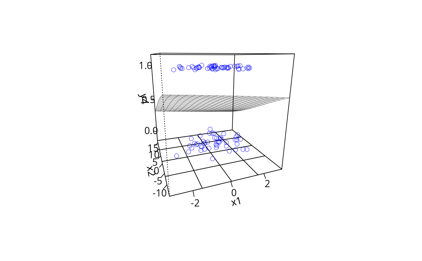
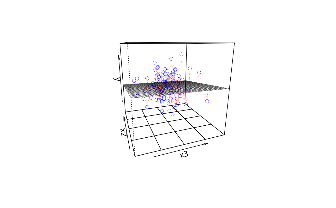
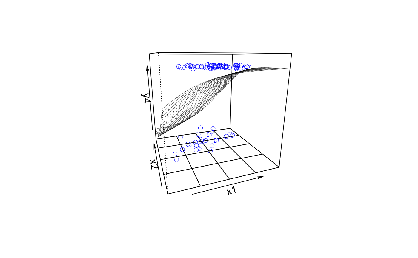
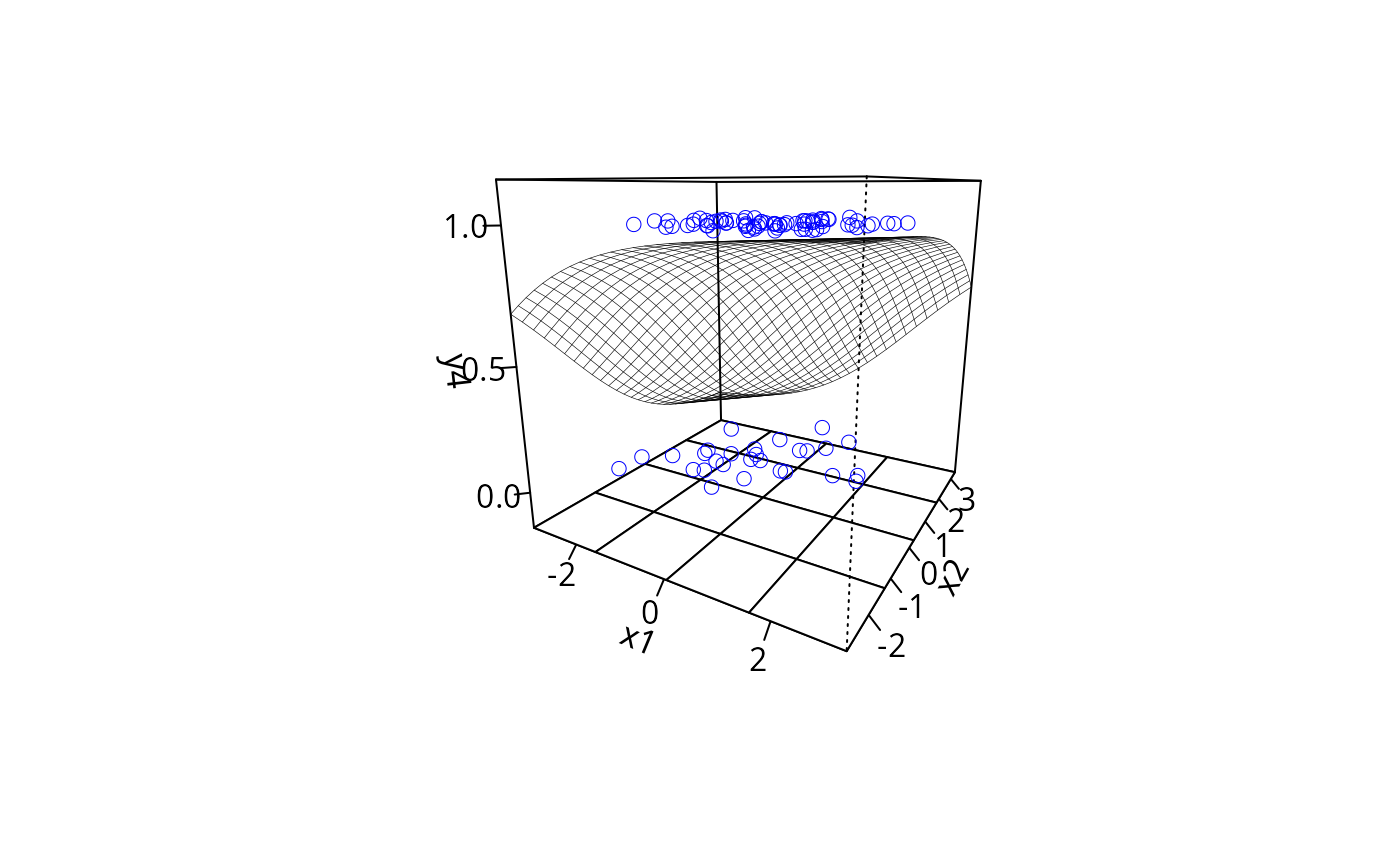
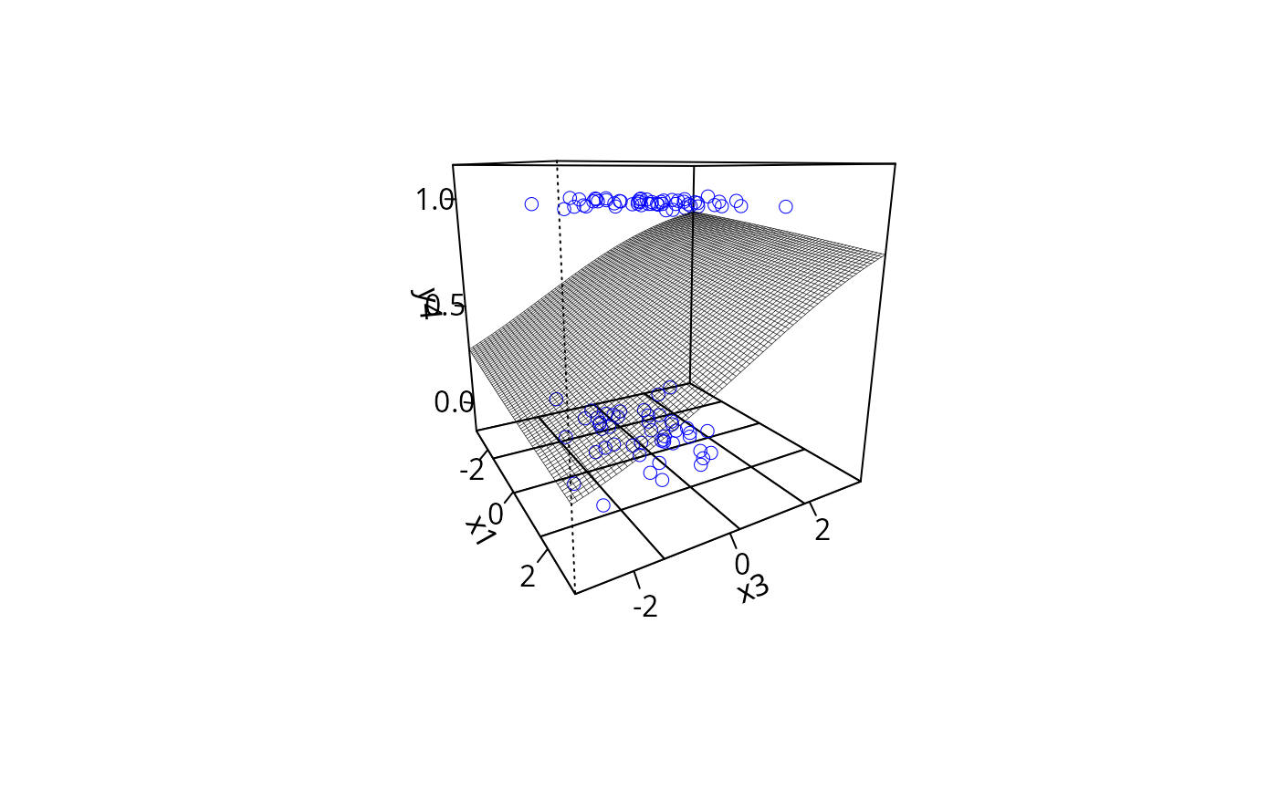
plotPlane(gm1, plotx1 = "x1", plotx2 = "x2")
eta3 <- 1.1 + .9*dat$x1 - .6*dat$x2 + .5*dat$x3
dat$y4 <- rbinom(100, size = 1, prob = exp( eta3)/(1+exp(eta3)))
gm1 <- glm(y4 ~ x1 + x2 + x3, data = dat, family = binomial(logit))
summary(gm1)
#>
#> Call:
#> glm(formula = y4 ~ x1 + x2 + x3, family = binomial(logit), data = dat)
#>
#> Coefficients:
#> Estimate Std. Error z value Pr(>|z|)
#> (Intercept) 1.03780 0.26082 3.979 6.92e-05 ***
#> x1 0.77932 0.24820 3.140 0.00169 **
#> x2 -0.77658 0.27490 -2.825 0.00473 **
#> x3 0.09249 0.26359 0.351 0.72568
#> ---
#> Signif. codes: 0 ‘***’ 0.001 ‘**’ 0.01 ‘*’ 0.05 ‘.’ 0.1 ‘ ’ 1
#>
#> (Dispersion parameter for binomial family taken to be 1)
#>
#> Null deviance: 118.59 on 99 degrees of freedom
#> Residual deviance: 100.34 on 96 degrees of freedom
#> AIC: 108.34
#>
#> Number of Fisher Scoring iterations: 5
#>
plotPlane(gm1, plotx1 = "x1", plotx2 = "x2")
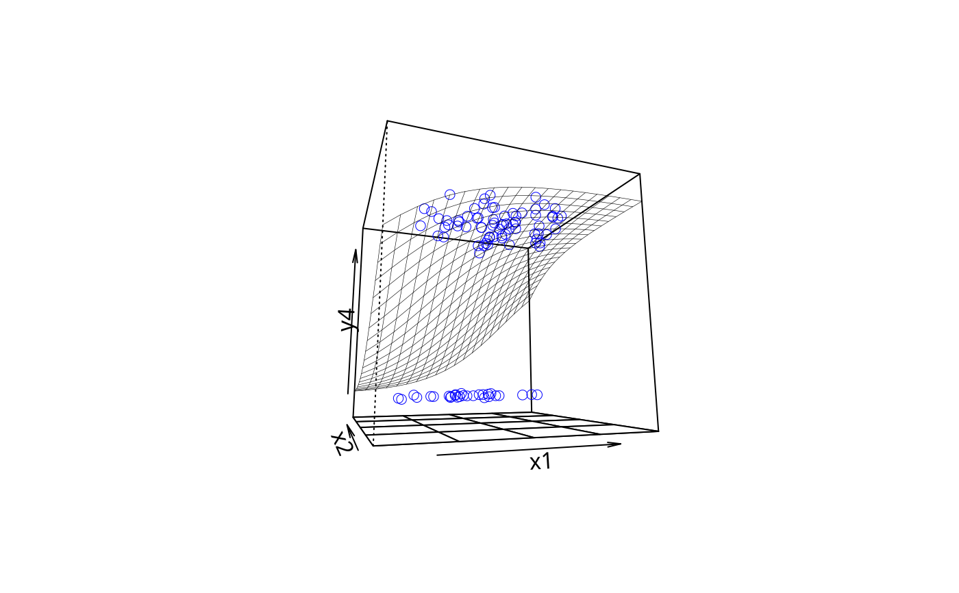
 plotPlane(gm1, plotx1 = "x1", plotx2 = "x2", phi = -10)
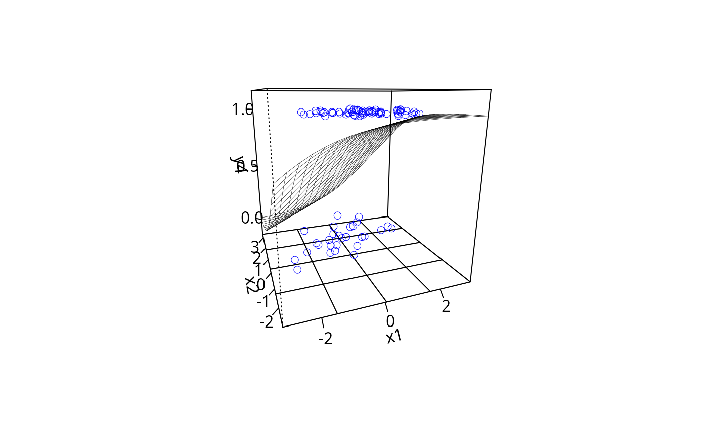
 plotPlane(gm1, plotx1 = "x1", plotx2 = "x2", ticktype = "detailed")
 plotPlane(gm1, plotx1 = "x1", plotx2 = "x2", ticktype = "detailed",
npp = 30, theta = 30)
plotPlane(gm1, plotx1 = "x1", plotx2 = "x2", ticktype = "detailed",
npp = 30, theta = 30)
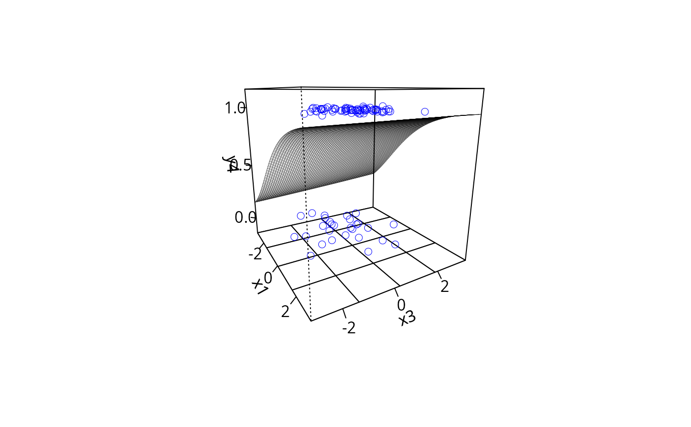
 plotPlane(gm1, plotx1 = "x1", plotx2 = "x3", ticktype = "detailed",
npp = 70, theta = 60)
plotPlane(gm1, plotx1 = "x1", plotx2 = "x3", ticktype = "detailed",
npp = 70, theta = 60)
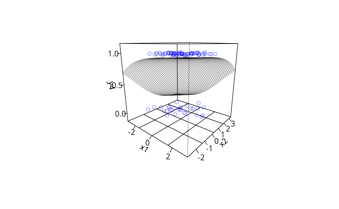
 plotPlane(gm1, plotx1 = "x1", plotx2 = "x2", ticktype = c("detailed"),
npp = 50, theta = 40)
plotPlane(gm1, plotx1 = "x1", plotx2 = "x2", ticktype = c("detailed"),
npp = 50, theta = 40)
 dat$x2 <- 5 * dat$x2
dat$x4 <- 10 * dat$x4
eta4 <- 0.1 + .15*dat$x1 - 0.1*dat$x2 + .25*dat$x3 + 0.1*dat$x4
dat$y4 <- rbinom(100, size = 1, prob = exp( eta4)/(1+exp(eta4)))
gm2 <- glm(y4 ~ x1 + x2 + x3 + x4, data = dat, family = binomial(logit))
summary(gm2)
#>
#> Call:
#> glm(formula = y4 ~ x1 + x2 + x3 + x4, family = binomial(logit),
#> data = dat)
#>
#> Coefficients:
#> Estimate Std. Error z value Pr(>|z|)
#> (Intercept) 0.08185 0.21891 0.374 0.7085
#> x1 -0.10840 0.19155 -0.566 0.5715
#> x2 -0.07264 0.04403 -1.650 0.0990 .
#> x3 0.47465 0.25320 1.875 0.0608 .
#> x4 0.05547 0.02526 2.196 0.0281 *
#> ---
#> Signif. codes: 0 ‘***’ 0.001 ‘**’ 0.01 ‘*’ 0.05 ‘.’ 0.1 ‘ ’ 1
#>
#> (Dispersion parameter for binomial family taken to be 1)
#>
#> Null deviance: 138.27 on 99 degrees of freedom
#> Residual deviance: 128.53 on 95 degrees of freedom
#> AIC: 138.53
#>
#> Number of Fisher Scoring iterations: 4
#>
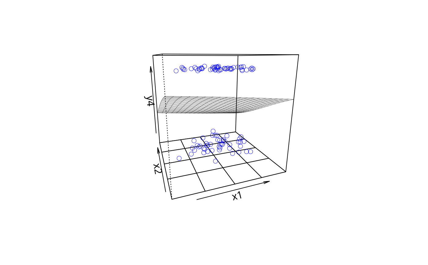
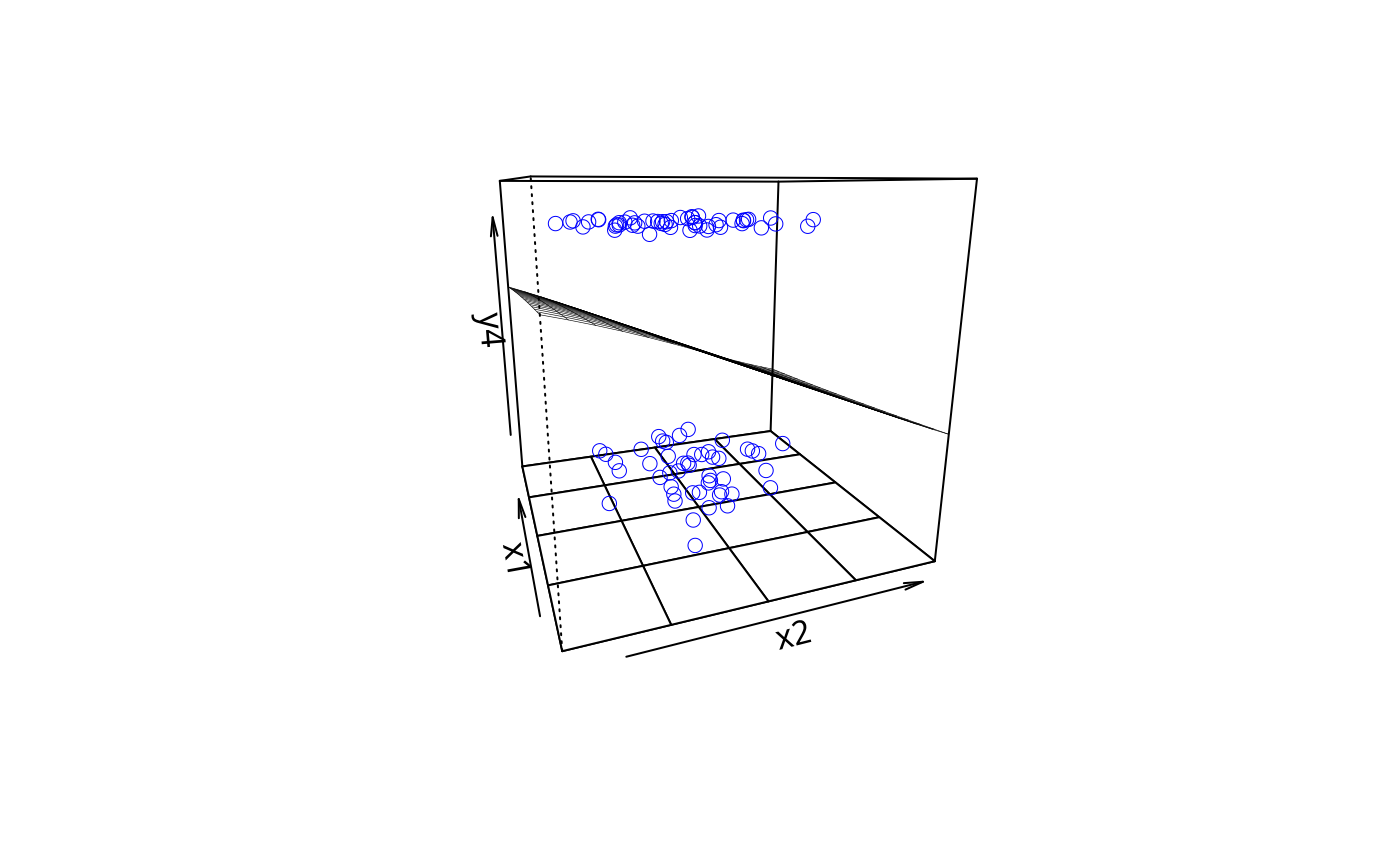
plotPlane(gm2, plotx1 = "x1", plotx2 = "x2")
dat$x2 <- 5 * dat$x2
dat$x4 <- 10 * dat$x4
eta4 <- 0.1 + .15*dat$x1 - 0.1*dat$x2 + .25*dat$x3 + 0.1*dat$x4
dat$y4 <- rbinom(100, size = 1, prob = exp( eta4)/(1+exp(eta4)))
gm2 <- glm(y4 ~ x1 + x2 + x3 + x4, data = dat, family = binomial(logit))
summary(gm2)
#>
#> Call:
#> glm(formula = y4 ~ x1 + x2 + x3 + x4, family = binomial(logit),
#> data = dat)
#>
#> Coefficients:
#> Estimate Std. Error z value Pr(>|z|)
#> (Intercept) 0.08185 0.21891 0.374 0.7085
#> x1 -0.10840 0.19155 -0.566 0.5715
#> x2 -0.07264 0.04403 -1.650 0.0990 .
#> x3 0.47465 0.25320 1.875 0.0608 .
#> x4 0.05547 0.02526 2.196 0.0281 *
#> ---
#> Signif. codes: 0 ‘***’ 0.001 ‘**’ 0.01 ‘*’ 0.05 ‘.’ 0.1 ‘ ’ 1
#>
#> (Dispersion parameter for binomial family taken to be 1)
#>
#> Null deviance: 138.27 on 99 degrees of freedom
#> Residual deviance: 128.53 on 95 degrees of freedom
#> AIC: 138.53
#>
#> Number of Fisher Scoring iterations: 4
#>
plotPlane(gm2, plotx1 = "x1", plotx2 = "x2")
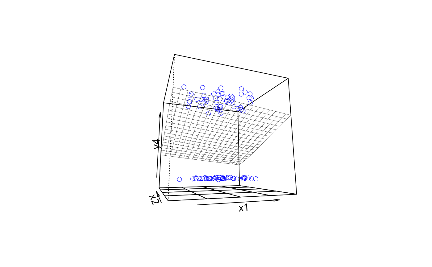
 plotPlane(gm2, plotx1 = "x2", plotx2 = "x1")
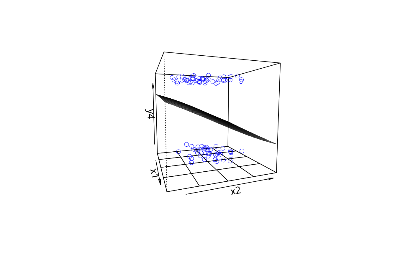
 plotPlane(gm2, plotx1 = "x1", plotx2 = "x2", phi = -10)
 plotPlane(gm2, plotx1 = "x1", plotx2 = "x2", phi = 5, theta = 70, npp = 40)
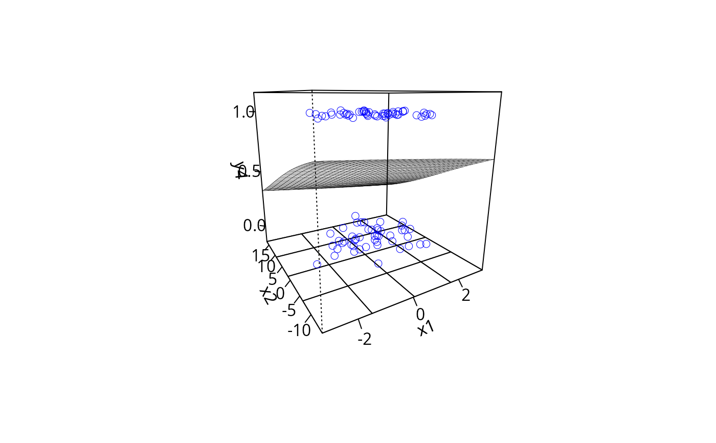
 plotPlane(gm2, plotx1 = "x1", plotx2 = "x2", ticktype = "detailed")
 plotPlane(gm2, plotx1 = "x1", plotx2 = "x2", ticktype = "detailed",
npp = 30, theta = -30)
plotPlane(gm2, plotx1 = "x1", plotx2 = "x2", ticktype = "detailed",
npp = 30, theta = -30)
 plotPlane(gm2, plotx1 = "x1", plotx2 = "x3", ticktype = "detailed",
npp = 70, theta = 60)
plotPlane(gm2, plotx1 = "x1", plotx2 = "x3", ticktype = "detailed",
npp = 70, theta = 60)
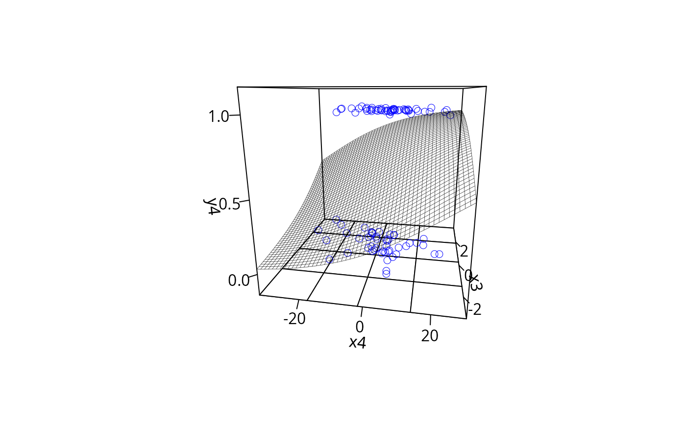
 plotPlane(gm2, plotx1 = "x4", plotx2 = "x3", ticktype = "detailed",
npp = 50, theta = 10)
plotPlane(gm2, plotx1 = "x4", plotx2 = "x3", ticktype = "detailed",
npp = 50, theta = 10)
 plotPlane(gm2, plotx1 = "x1", plotx2 = "x2", ticktype = c("detailed"))