Superimpose regression lines on a plotted plane
addLines.RdThe examples will demonstrate the intended usage.
Details
From an educational stand point, the objective is to assist with the student's conceptualization of the two and three dimensional regression relationships.
Author
Paul E. Johnson pauljohn@ku.edu
Examples
##library(rockchalk)
set.seed(12345)
dfadd <- genCorrelatedData2(100, means = c(0,0,0,0), sds = 1, rho = 0,
beta = c(0.03, 0.01, 0.1, 0.4, -0.1), stde = 2)
#> [1] "The equation that was calculated was"
#> y = 0.03 + 0.01*x1 + 0.1*x2 + 0.4*x3 + -0.1*x4
#> + 0*x1*x1 + 0*x2*x1 + 0*x3*x1 + 0*x4*x1
#> + 0*x1*x2 + 0*x2*x2 + 0*x3*x2 + 0*x4*x2
#> + 0*x1*x3 + 0*x2*x3 + 0*x3*x3 + 0*x4*x3
#> + 0*x1*x4 + 0*x2*x4 + 0*x3*x4 + 0*x4*x4
#> + N(0,2) random error
dfadd$xcat1 <- gl(2,50, labels=c("M","F"))
dfadd$xcat2 <- cut(rnorm(100), breaks=c(-Inf, 0, 0.4, 0.9, 1, Inf),
labels=c("R", "M", "D", "P", "G"))
dfadd$y2 <- 0.03 + 0.1*dfadd$x1 + 0.1*dfadd$x2 +
0.25*dfadd$x1*dfadd$x2 + 0.4*dfadd$x3 - 0.1*dfadd$x4 +
0.2 * as.numeric(dfadd$xcat1) +
contrasts(dfadd$xcat2)[as.numeric(dfadd$xcat2), ] %*% c(-0.1, 0.1, 0.2, 0) +
1 * rnorm(100)
summarize(dfadd)
#> Numeric variables
#> y x1 x2 x3 x4 y2
#> min -4.992 -2.347 -2.135 -2.380 -2.582 -2.621
#> med 0.080 0.288 0.090 0.019 0.287 0.258
#> max 4.577 2.477 2.747 2.331 2.484 3.330
#> mean -0.069 0.196 0.119 -0.007 0.152 0.331
#> sd 1.813 0.989 0.999 1.067 0.999 1.176
#> skewness -0.220 0.067 0.296 -0.082 -0.356 -0.038
#> kurtosis -0.004 -0.395 0.020 -0.510 0.046 -0.498
#> nobs 100 100 100 100 100 100
#> nmissing 0 0 0 0 0 0
#>
#> Nonnumeric variables
#> xcat1 xcat2
#> M: 50 R: 47
#> F: 50 M: 11
#> D: 26
#> G: 16
#> nobs : 100 nobs : 100.000
#> nmiss : 0 nmiss : 0.000
#> entropy : 1 entropy : 1.791
#> normedEntropy: 1 normedEntropy: 0.895
## linear ordinary regression
m1 <- lm(y ~ x1 + x2 + x3 + x4, data = dfadd)
summary(m1)
#>
#> Call:
#> lm(formula = y ~ x1 + x2 + x3 + x4, data = dfadd)
#>
#> Residuals:
#> Min 1Q Median 3Q Max
#> -4.5658 -1.2619 0.1185 1.1209 4.0642
#>
#> Coefficients:
#> Estimate Std. Error t value Pr(>|t|)
#> (Intercept) -0.04169 0.17971 -0.232 0.81706
#> x1 0.17428 0.17759 0.981 0.32891
#> x2 -0.38871 0.17498 -2.221 0.02870 *
#> x3 0.46476 0.16374 2.838 0.00554 **
#> x4 -0.07608 0.17370 -0.438 0.66238
#> ---
#> Signif. codes: 0 ‘***’ 0.001 ‘**’ 0.01 ‘*’ 0.05 ‘.’ 0.1 ‘ ’ 1
#>
#> Residual standard error: 1.724 on 95 degrees of freedom
#> Multiple R-squared: 0.1324, Adjusted R-squared: 0.09585
#> F-statistic: 3.624 on 4 and 95 DF, p-value: 0.008575
#>
mcDiagnose(m1)
#> The following auxiliary models are being estimated and returned in a list:
#> x1 ~ x2 + x3 + x4
#> x2 ~ x1 + x3 + x4
#> x3 ~ x1 + x2 + x4
#> x4 ~ x1 + x2 + x3
#>
#> R_j Squares of auxiliary models
#> x1 x2 x3 x4
#> 0.026650999 0.017226201 0.015773844 0.003202144
#> The Corresponding VIF, 1/(1-R_j^2)
#> x1 x2 x3 x4
#> 1.027381 1.017528 1.016027 1.003212
#> Bivariate Pearson Correlations for design matrix
#> x1 x2 x3 x4
#> x1 1.00 -0.11 -0.12 0.00
#> x2 -0.11 1.00 -0.03 -0.05
#> x3 -0.12 -0.03 1.00 0.02
#> x4 0.00 -0.05 0.02 1.00
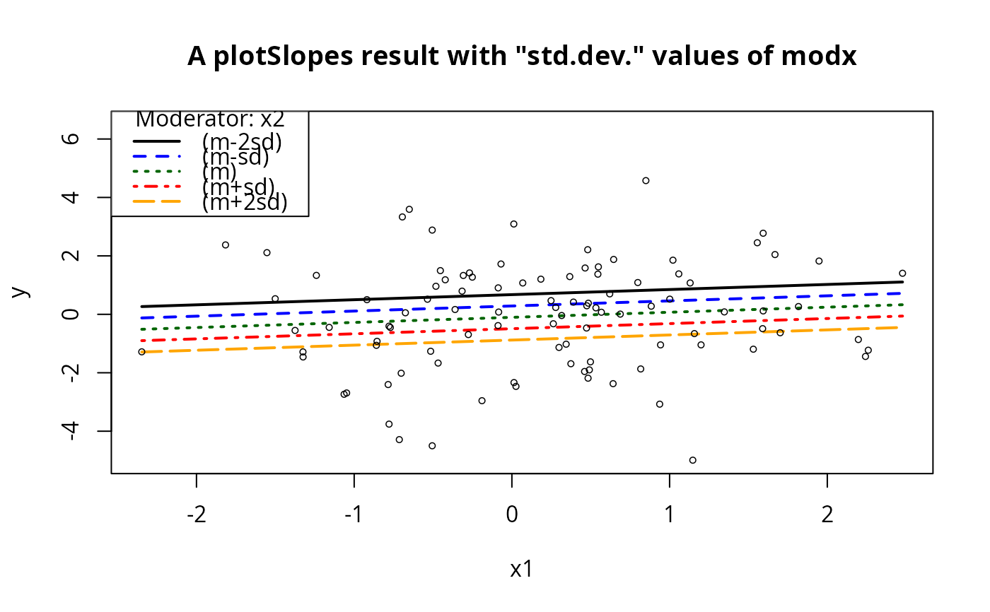
## These will be parallel lines
plotSlopes(m1, plotx = "x1", modx = "x2", modxVals = "std.dev.",
n = 5, main = "A plotSlopes result with \"std.dev.\" values of modx")
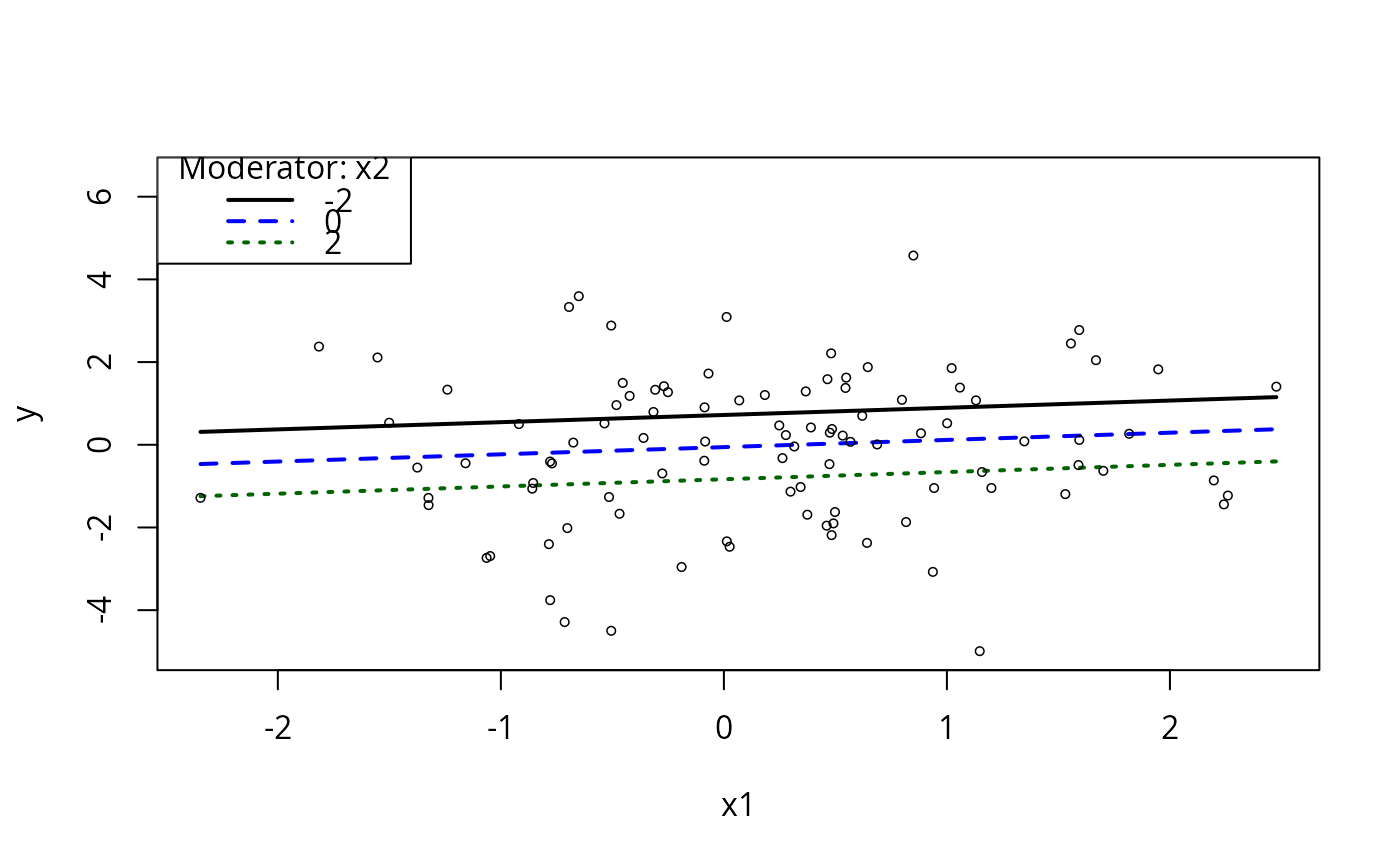
 m1ps <- plotSlopes(m1, plotx = "x1", modx = "x2", modxVals = c(-2,0,2))
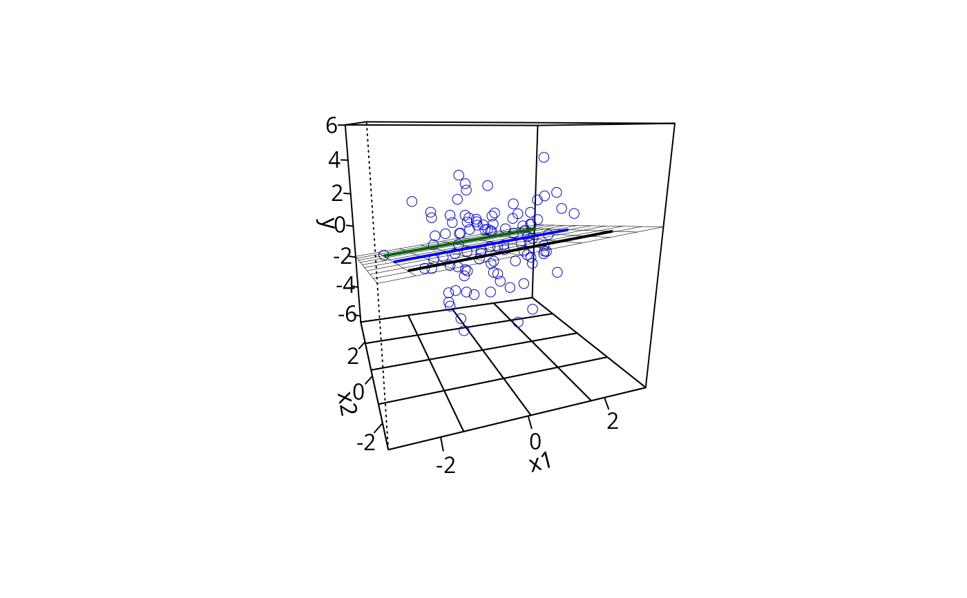
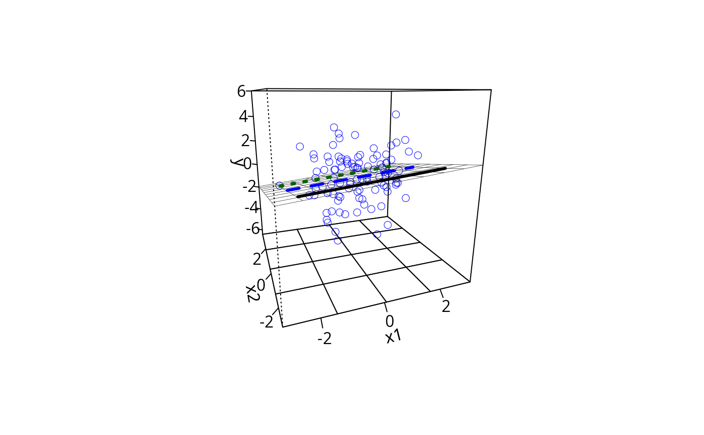
 m1pp <- plotPlane(m1, plotx1 = "x1", plotx2 = "x2",
ticktype = "detailed", npp = 10)
addLines(from = m1ps, to = m1pp, lty = 1, lwd = 2)
m1pp <- plotPlane(m1, plotx1 = "x1", plotx2 = "x2",
ticktype = "detailed", npp = 10)
addLines(from = m1ps, to = m1pp, lty = 1, lwd = 2)
 #> NULL
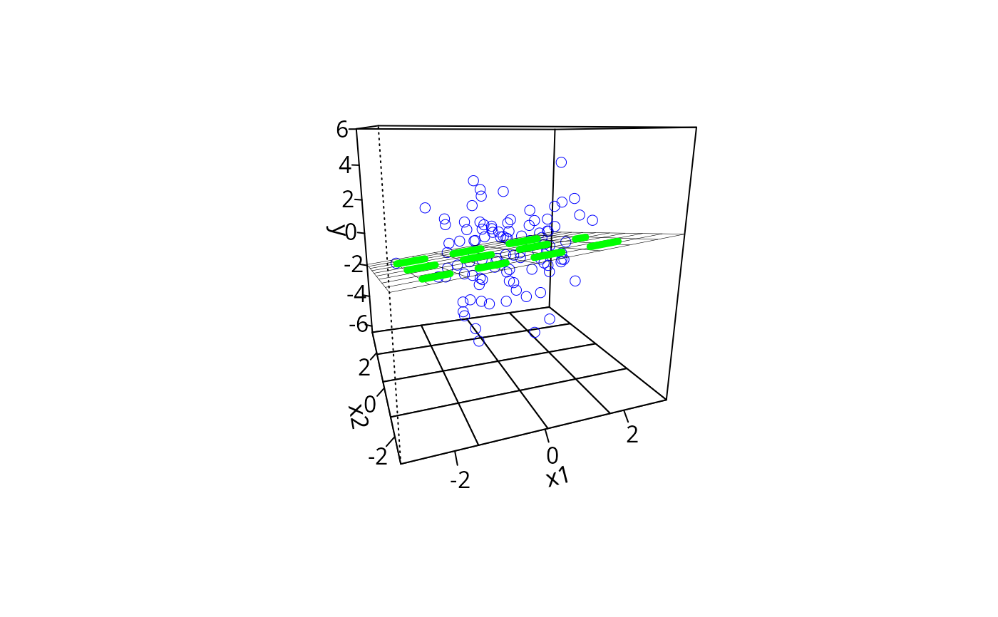
m1pp <- plotPlane(m1, plotx1 = "x1", plotx2 = "x2", ticktype = "detailed",
npp = 10)
addLines(from = m1ps, to = m1pp, lty = 2, lwd = 5, col = "green")
#> NULL
m1pp <- plotPlane(m1, plotx1 = "x1", plotx2 = "x2", ticktype = "detailed",
npp = 10)
addLines(from = m1ps, to = m1pp, lty = 2, lwd = 5, col = "green")
 #> NULL
## Other approach would wrap same into the linesFrom argument in plotPlane
plotPlane(m1, plotx1 = "x1", plotx2 = "x2", ticktype = "detailed",
npp = 10, linesFrom = m1ps)
#> NULL
## Other approach would wrap same into the linesFrom argument in plotPlane
plotPlane(m1, plotx1 = "x1", plotx2 = "x2", ticktype = "detailed",
npp = 10, linesFrom = m1ps)
 ## Need to think more on whether dotted lines from ps object should
## be converted to solid lines in plotPlane.
## Need to think more on whether dotted lines from ps object should
## be converted to solid lines in plotPlane.