Validate Predicted Probabilities Against Observed Survival Times
val.surv.RdThe val.surv function is useful for validating predicted survival
probabilities against right-censored failure times. If u is
specified, the hazard regression function hare in the
polspline package is used to relate predicted survival
probability at time u to observed survival times (and censoring
indicators) to estimate the actual survival probability at time
u as a function of the estimated survival probability at that
time, est.surv. If est.surv is not given, fit must
be specified and the survest function is used to obtain the
predicted values (using newdata if it is given, or using the
stored linear predictor values if not). hare or movStats
(when method="smoothkm") is given the sole
predictor fun(est.surv) where fun is given by the user or
is inferred from fit. fun is the function of predicted
survival probabilities that one expects to create a linear relationship
with the linear predictors.
hare uses an adaptive procedure to find a linear spline of
fun(est.surv) in a model where the log hazard is a linear spline
in time \(t\), and cross-products between the two splines are allowed so as to
not assume proportional hazards. Thus hare assumes that the
covariate and time functions are smooth but not much else, if the number
of events in the dataset is large enough for obtaining a reliable
flexible fit. Or specify method="smoothkm" to use the Hmisc movStats
function to compute smoothed (by default using supsmu)
moving window Kaplan-Meier estimates. This method is more flexible than hare.
There are special print and plot methods
when u is given. In this case, val.surv returns an object
of class "val.survh", otherwise it returns an object of class
"val.surv".
If u is not specified, val.surv uses Cox-Snell (1968)
residuals on the cumulative
probability scale to check on the calibration of a survival model
against right-censored failure time data. If the predicted survival
probability at time \(t\) for a subject having predictors \(X\) is
\(S(t|X)\), this method is based on the fact that the predicted
probability of failure before time \(t\), \(1 - S(t|X)\), when
evaluated at the subject's actual survival time \(T\), has a uniform
(0,1) distribution. The quantity \(1 - S(T|X)\) is right-censored
when \(T\) is. By getting one minus the Kaplan-Meier estimate of the
distribution of \(1 - S(T|X)\) and plotting against the 45 degree line
we can check for calibration accuracy. A more stringent assessment can
be obtained by stratifying this analysis by an important predictor
variable. The theoretical uniform distribution is only an approximation
when the survival probabilities are estimates and not population values.
When censor is specified to val.surv, a different
validation is done that is more stringent but that only uses the
uncensored failure times. This method is used for type I censoring when
the theoretical censoring times are known for subjects having uncensored
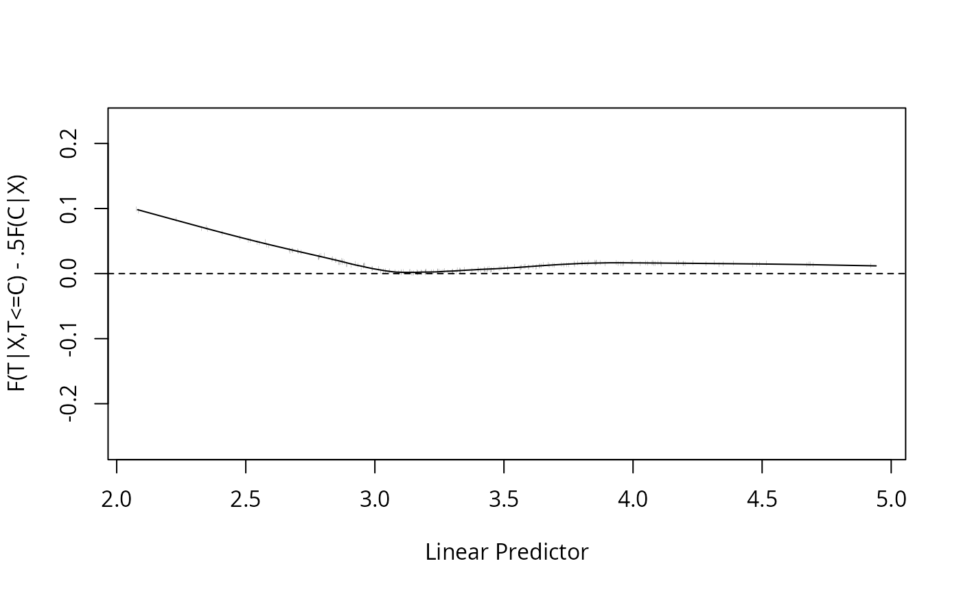
failure times. Let \(T\), \(C\), and \(F\) denote respectively
the failure time, censoring time, and cumulative failure time
distribution (\(1 - S\)). The expected value of \(F(T | X)\) is 0.5
when \(T\) represents the subject's actual failure time. The expected
value for an uncensored time is the expected value of \(F(T | T \leq
C, X) = 0.5 F(C | X)\). A smooth plot of \(F(T|X) - 0.5 F(C|X)\) for
uncensored \(T\) should be a flat line through \(y=0\) if the model
is well calibrated. A smooth plot of \(2F(T|X)/F(C|X)\) for
uncensored \(T\) should be a flat line through \(y=1.0\). The smooth
plot is obtained by smoothing the (linear predictor, difference or
ratio) pairs.
Note that the Cox-Snell residual plot is not very sensitive to model lack of fit.
Usage
val.surv(fit, newdata, S, est.surv,
         method=c('hare', 'smoothkm'),
         censor, u, fun, lim, evaluate=100, pred, maxdim=5, ...)

# S3 method for class 'val.survh'
print(x, ...)

# S3 method for class 'val.survh'
plot(x, lim, xlab, ylab,
                         riskdist=TRUE, add=FALSE,
                         scat1d.opts=list(nhistSpike=200), ...)

# S3 method for class 'val.surv'
plot(x, group, g.group=4,
     what=c('difference','ratio'),
     type=c('l','b','p'),
     xlab, ylab, xlim, ylim, datadensity=TRUE, ...)
Arguments
- fit
a fit object created by
cphorpsm- newdata
a data frame for which
val.survshould obtain predicted survival probabilities. If omitted, survival estimates are made for all of the subjects used infit.- S
- est.surv
a vector of estimated survival probabilities corresponding to times in the first column of
S.- method
applies if
uis specified and defaults tohare- censor
a vector of censoring times. Only the censoring times for uncensored observations are used.
- u
a single numeric follow-up time
- fun
a function that transforms survival probabilities into the scale of the linear predictor. If
fitis given, and represents either a Cox, Weibull, or exponential fit,funis automatically set to log(-log(p)).- lim
a 2-vector specifying limits of predicted survival probabilities for obtaining estimated actual probabilities at time
u. Default forval.survis the limits for predictions fromdatadist, which for large \(n\) is the 10th smallest and 10th largest predicted survival probability. Forplot.val.survh, the default forlimis the range of the combination of predicted probabilities and calibrated actual probabilities.limis used for both axes of the calibration plot.- evaluate
the number of evenly spaced points over the range of predicted probabilities. This defines the points at which calibrated predictions are obtained for plotting.
- pred
a vector of points at which to evaluate predicted probabilities, overriding
lim- maxdim
see
hare- x
result of
val.surv- xlab
x-axis label. For
plot.survh, defaults forxlabandylabcome fromuand the units of measurement for the raw survival times.- ylab
y-axis label
- riskdist
set to
FALSEto not callscat1dto draw the distribution of predicted (uncalibrated) probabilities- add
set to
TRUEif adding to an existing plot- scat1d.opts
a
listof options to pass toscat1d. By default, the optionnhistSpike=200is passed so that a spike histogram is used if the sample size exceeds 200.- ...
When
uis given toval.surv, ... represents optional arguments tohareormovStats. It can represent arguments to pass toplotorlinesforplot.val.survh. Otherwise, ... contains optional arguments forplsmoorplot. Forprint.val.survh, ... is ignored.- group
a grouping variable. If numeric this variable is grouped into
g.groupquantile groups (default is quartiles).group,g.group,what, andtypeapply whenuis not given.- g.group
number of quantile groups to use when
groupis given and variable is numeric.- what
the quantity to plot when
censorwas in effect. The default is to show the difference between cumulative probabilities and their expectation given the censoring time. Setwhat="ratio"to show the ratio instead.- type
Set to the default (
"l") to plot the trend line only,"b"to plot both individual subjects ratios and trend lines, or"p"to plot only points.- xlim,ylim
axis limits for
plot.val.survwhen thecensorvariable was used.- datadensity
By default,
plot.val.survwill show the data density on each curve that is created as a result ofcensorbeing present. Setdatadensity=FALSEto suppress these tick marks drawn byscat1d.
References
Cox DR, Snell EJ (1968):A general definition of residuals (with discussion). JRSSB 30:248–275.
Kooperberg C, Stone C, Truong Y (1995): Hazard regression. JASA 90:78–94.
May M, Royston P, Egger M, Justice AC, Sterne JAC (2004):Development and validation of a prognostic model for survival time data: application to prognosis of HIV positive patients treated with antiretroviral therapy. Stat in Med 23:2375–2398.
Stallard N (2009): Simple tests for th external validation of mortality prediction scores. Stat in Med 28:377–388.
Examples
# Generate failure times from an exponential distribution
require(survival)
set.seed(123) # so can reproduce results
n <- 1000
age <- 50 + 12*rnorm(n)
sex <- factor(sample(c('Male','Female'), n, rep=TRUE, prob=c(.6, .4)))
cens <- 15*runif(n)
h <- .02*exp(.04*(age-50)+.8*(sex=='Female'))
t <- -log(runif(n))/h
units(t) <- 'Year'
label(t) <- 'Time to Event'
ev <- ifelse(t <= cens, 1, 0)
t <- pmin(t, cens)
S <- Surv(t, ev)
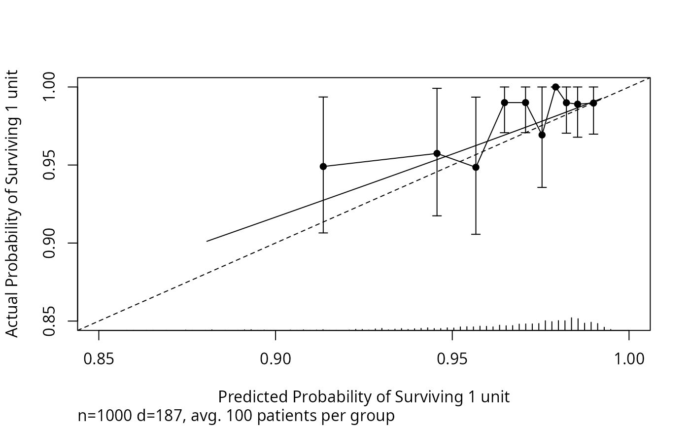
# First validate true model used to generate data
# If hare is available, make a smooth calibration plot for 1-year
# survival probability where we predict 1-year survival using the
# known true population survival probability
# In addition, use groupkm to show that grouping predictions into
# intervals and computing Kaplan-Meier estimates is not as accurate.
s1 <- exp(-h*1)
w <- val.surv(est.surv=s1, S=S, u=1,
fun=function(p)log(-log(p)))
plot(w, lim=c(.85,1), scat1d.opts=list(nhistSpike=200, side=1))
groupkm(s1, S, m=100, u=1, pl=TRUE, add=TRUE)
 #> x n events KM std.err
#> [1,] 0.913 100 41 0.949 0.0234
#> [2,] 0.946 100 29 0.957 0.0218
#> [3,] 0.957 100 24 0.949 0.0236
#> [4,] 0.965 100 22 0.990 0.0101
#> [5,] 0.971 100 19 0.990 0.0101
#> [6,] 0.975 100 14 0.969 0.0180
#> [7,] 0.979 100 10 1.000 0.0000
#> [8,] 0.982 100 12 0.990 0.0102
#> [9,] 0.985 100 9 0.989 0.0110
#> [10,] 0.990 100 7 0.990 0.0104
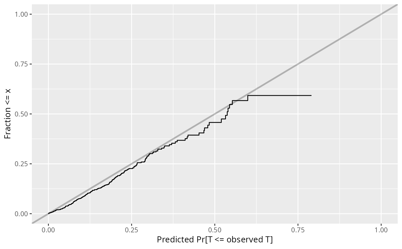
# Now validate the true model using residuals
w <- val.surv(est.surv=exp(-h*t), S=S)
plot(w)
#> x n events KM std.err
#> [1,] 0.913 100 41 0.949 0.0234
#> [2,] 0.946 100 29 0.957 0.0218
#> [3,] 0.957 100 24 0.949 0.0236
#> [4,] 0.965 100 22 0.990 0.0101
#> [5,] 0.971 100 19 0.990 0.0101
#> [6,] 0.975 100 14 0.969 0.0180
#> [7,] 0.979 100 10 1.000 0.0000
#> [8,] 0.982 100 12 0.990 0.0102
#> [9,] 0.985 100 9 0.989 0.0110
#> [10,] 0.990 100 7 0.990 0.0104
# Now validate the true model using residuals
w <- val.surv(est.surv=exp(-h*t), S=S)
plot(w)
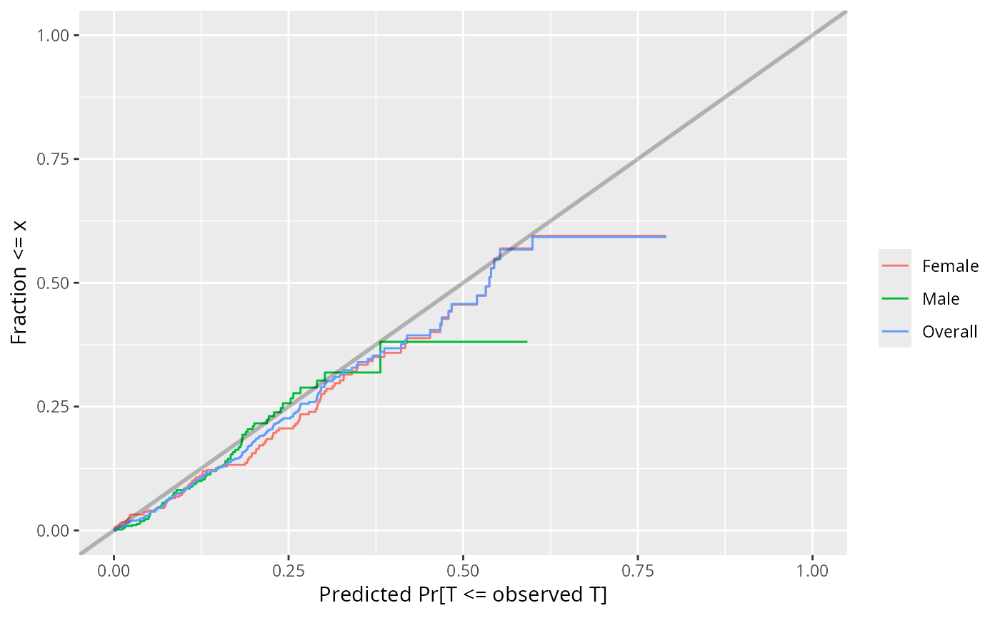
 plot(w, group=sex) # stratify by sex
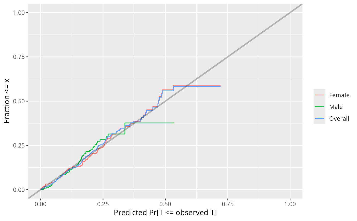
 # Now fit an exponential model and validate
# Note this is not really a validation as we're using the
# training data here
f <- psm(S ~ age + sex, dist='exponential', y=TRUE)
w <- val.surv(f)
plot(w, group=sex)
# Now fit an exponential model and validate
# Note this is not really a validation as we're using the
# training data here
f <- psm(S ~ age + sex, dist='exponential', y=TRUE)
w <- val.surv(f)
plot(w, group=sex)
 # We know the censoring time on every subject, so we can
# compare the predicted Pr[T <= observed T | T>c, X] to
# its expectation 0.5 Pr[T <= C | X] where C = censoring time
# We plot a ratio that should equal one
w <- val.surv(f, censor=cens)
plot(w)
# We know the censoring time on every subject, so we can
# compare the predicted Pr[T <= observed T | T>c, X] to
# its expectation 0.5 Pr[T <= C | X] where C = censoring time
# We plot a ratio that should equal one
w <- val.surv(f, censor=cens)
plot(w)
 #> Mean F(T|T<C,X) Expected
#> [1,] 0.155 0.145
plot(w, group=age, g=3) # stratify by tertile of age
#> Mean F(T|T<C,X) Expected
#> [1,] 0.155 0.145
plot(w, group=age, g=3) # stratify by tertile of age
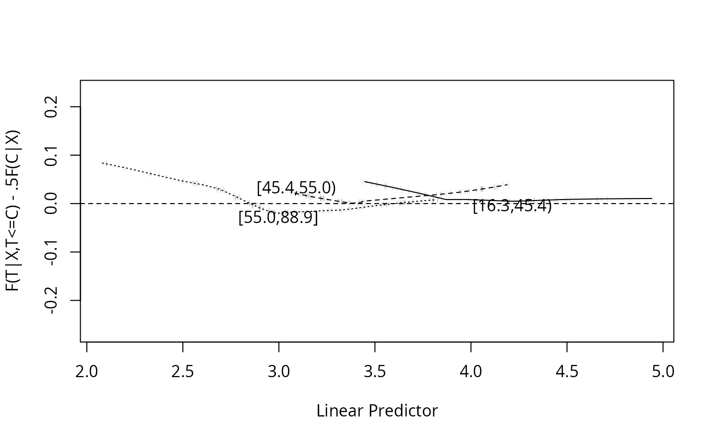 #> Mean F(T|T<C,X) Expected
#> [16.3,45.4) 0.106 0.0871
#> [45.4,55.0) 0.132 0.1179
#> [55.0,88.9] 0.188 0.1857
#> Mean F(T|T<C,X) Expected
#> [16.3,45.4) 0.106 0.0871
#> [45.4,55.0) 0.132 0.1179
#> [55.0,88.9] 0.188 0.1857