Cox Proportional Hazards Model and Extensions

Modification of Therneau's coxph function to fit the Cox model and its extension, the Andersen-Gill model. The latter allows for interval time-dependent covariables, time-dependent strata, and repeated events. The Survival method for an object created by cph returns an S function for computing estimates of the survival function. The Quantile method for cph returns an S function for computing quantiles of survival time (median, by default). The Mean method returns a function for computing the mean survival time. This function issues a warning if the last follow-up time is uncensored, unless a restricted mean is explicitly requested.

Usage

cph(formula = formula(data), data=environment(formula),
    weights, subset, na.action=na.delete, 
    method=c("efron","breslow","exact","model.frame","model.matrix"), 
    singular.ok=FALSE, robust=FALSE,
    model=FALSE, x=FALSE, y=FALSE, se.fit=FALSE,
    linear.predictors=TRUE, residuals=TRUE, nonames=FALSE,
    eps=1e-4, init, iter.max=10, tol=1e-9, surv=FALSE, time.inc,
    type=NULL, vartype=NULL, debug=FALSE, ...)

# S3 method for class 'cph'
Survival(object, ...)
# Evaluate result as g(times, lp, stratum=1, type=c("step","polygon"))

# S3 method for class 'cph'
Quantile(object, ...)
# Evaluate like h(q, lp, stratum=1, type=c("step","polygon"))

# S3 method for class 'cph'
Mean(object, method=c("exact","approximate"), type=c("step","polygon"),
          n=75, tmax, ...)
# E.g. m(lp, stratum=1, type=c("step","polygon"), tmax, \dots)

Arguments

formula

an S formula object with a Surv object on the left-hand side. The terms can specify any S model formula with up to third-order interactions. The strat function may appear in the terms, as a main effect or an interacting factor. To stratify on both race and sex, you would include both terms strat(race) and strat(sex). Stratification factors may interact with non-stratification factors; not all stratification terms need interact with the same modeled factors.

object

an object created by cph with surv=TRUE

data

name of an S data frame containing all needed variables. Omit this to use a data frame already in the S “search list”.

weights

case weights

subset

an expression defining a subset of the observations to use in the fit. The default is to use all observations. Specify for example age>50 & sex="male" or c(1:100,200:300) respectively to use the observations satisfying a logical expression or those having row numbers in the given vector.

na.action

specifies an S function to handle missing data. The default is the function na.delete, which causes observations with any variable missing to be deleted. The main difference between na.delete and the S-supplied function na.omit is that na.delete makes a list of the number of observations that are missing on each variable in the model. The na.action is usally specified by e.g. options(na.action="na.delete").

method

for cph, specifies a particular fitting method, "model.frame" instead to return the model frame of the predictor and response variables satisfying any subset or missing value checks, or "model.matrix" to return the expanded design matrix. The default is "efron", to use Efron's likelihood for fitting the model.

For Mean.cph, method is "exact" to use numerical integration of the survival function at any linear predictor value to obtain a mean survival time. Specify method="approximate" to use an approximate method that is slower when Mean.cph is executing but then is essentially instant thereafter. For the approximate method, the area is computed for n points equally spaced between the min and max observed linear predictor values. This calculation is done separately for each stratum. Then the n pairs (X beta, area) are saved in the generated S function, and when this function is evaluated, the approx function is used to evaluate the mean for any given linear predictor values, using linear interpolation over the n X beta values.

singular.ok

If TRUE, the program will automatically skip over columns of the X matrix that are linear combinations of earlier columns. In this case the coefficients for such columns will be NA, and the variance matrix will contain zeros. For ancillary calculations, such as the linear predictor, the missing coefficients are treated as zeros. The singularities will prevent many of the features of the rms library from working.

robust

if TRUE a robust variance estimate is returned. Default is TRUE if the model includes a cluster() operative, FALSE otherwise.

model

default is FALSE(false). Set to TRUE to return the model frame as element model of the fit object.

x

default is FALSE. Set to TRUE to return the expanded design matrix as element x (without intercept indicators) of the returned fit object.

y

default is FALSE. Set to TRUE to return the vector of response values (Surv object) as element y of the fit.

se.fit

default is FALSE. Set to TRUE to compute the estimated standard errors of the estimate of X beta and store them in element se.fit of the fit. The predictors are first centered to their means before computing the standard errors.

linear.predictors

set to FALSE to omit linear.predictors vector from fit

residuals

set to FALSE to omit residuals vector from fit

nonames

set to TRUE to not set names attribute for linear.predictors, residuals, se.fit, and rows of design matrix

eps

convergence criterion - change in log likelihood.

init

vector of initial parameter estimates. Defaults to all zeros. Special residuals can be obtained by setting some elements of init to MLEs and others to zero and specifying iter.max=1.

iter.max

maximum number of iterations to allow. Set to 0 to obtain certain null-model residuals.

tol

tolerance for declaring singularity for matrix inversion (available only when survival5 or later package is in effect)

surv

set to TRUE to compute underlying survival estimates for each stratum, and to store these along with standard errors of log Lambda(t), maxtime (maximum observed survival or censoring time), and surv.summary in the returned object. Set surv="summary" to only compute and store surv.summary, not survival estimates at each unique uncensored failure time. If you specify x=TRUE and y=TRUE, you can obtain predicted survival later, with accurate confidence intervals for any set of predictor values. The standard error information stored as a result of surv=TRUE are only accurate at the mean of all predictors. If the model has no covariables, these are of course OK. The main reason for using surv is to greatly speed up the computation of predicted survival probabilities as a function of the covariables, when accurate confidence intervals are not needed.

time.inc

time increment used in deriving surv.summary. Survival, number at risk, and standard error will be stored for t=0, time.inc, 2 time.inc, ..., maxtime, where maxtime is the maximum survival time over all strata. time.inc is also used in constructing the time axis in the survplot function (see below). The default value for time.inc is 30 if units(ftime) = "Day" or no units attribute has been attached to the survival time variable. If units(ftime) is a word other than "Day", the default for time.inc is 1 when it is omitted, unless maxtime<1, then maxtime/10 is used as time.inc. If time.inc is not given and maxtime/ default time.inc > 25, time.inc is increased.

type

(for cph) applies if surv is TRUE or "summary". If type is omitted, the method consistent with method is used. See survfit.coxph (under survfit) or survfit.cph for details and for the definitions of values of type

For Survival, Quantile, Mean set to "polygon" to use linear interpolation instead of the usual step function. For Mean, the default of step will yield the sample mean in the case of no censoring and no covariables, if type="kaplan-meier" was specified to cph. For method="exact", the value of type is passed to the generated function, and it can be overridden when that function is actually invoked. For method="approximate", Mean.cph generates the function different ways according to type, and this cannot be changed when the function is actually invoked.

vartype

see survfit.coxph

debug

set to TRUE to print debugging information related to model matrix construction. You can also use options(debug=TRUE).

...

other arguments passed to coxph.fit from cph. Ignored by other functions.

times

a scalar or vector of times at which to evaluate the survival estimates

lp

a scalar or vector of linear predictors (including the centering constant) at which to evaluate the survival estimates

stratum

a scalar stratum number or name (e.g., "sex=male") to use in getting survival probabilities

q

a scalar quantile or a vector of quantiles to compute

n

the number of points at which to evaluate the mean survival time, for method="approximate" in Mean.cph.

tmax

For Mean.cph, the default is to compute the overall mean (and produce a warning message if there is censoring at the end of follow-up). To compute a restricted mean life length, specify the truncation point as tmax. For method="exact", tmax is passed to the generated function and it may be overridden when that function is invoked. For method="approximate", tmax must be specified at the time that Mean.cph is run.

Value

For Survival, Quantile, or Mean, an S function is returned. Otherwise, in addition to what is listed below, formula/design information and the components maxtime, time.inc, units, model, x, y, se.fit are stored, the last 5 depending on the settings of options by the same names. The vectors or matrix stored if y=TRUE or x=TRUE have rows deleted according to subset and to missing data, and have names or row names that come from the data frame used as input data.

n: table with one row per stratum containing number of censored and uncensored observations
coef: vector of regression coefficients
stats: vector containing the named elements Obs, Events, Model L.R., d.f., P, Score, Score P, R2, Somers' Dxy, g-index, and gr, the g-index on the hazard ratio scale. R2 is the Nagelkerke R-squared, with division by the maximum attainable R-squared.
var: variance/covariance matrix of coefficients
linear.predictors: values of predicted X beta for observations used in fit, normalized to have overall mean zero, then having any offsets added
resid: martingale residuals
loglik: log likelihood at initial and final parameter values
score: value of score statistic at initial values of parameters
times: lists of times (if surv="T")
surv: lists of underlying survival probability estimates
std.err: lists of standard errors of estimate log-log survival
surv.summary: a 3 dimensional array if surv=TRUE. The first dimension is time ranging from 0 to maxtime by time.inc. The second dimension refers to strata. The third dimension contains the time-oriented matrix with Survival, n.risk (number of subjects at risk), and std.err (standard error of log-log survival).
center: centering constant, equal to overall mean of X beta.

Details

If there is any strata by covariable interaction in the model such that the mean X beta varies greatly over strata, method="approximate" may not yield very accurate estimates of the mean in Mean.cph.

For method="approximate" if you ask for an estimate of the mean for a linear predictor value that was outside the range of linear predictors stored with the fit, the mean for that observation will be NA.

Author

Frank Harrell
Department of Biostatistics, Vanderbilt University
fh@fharrell.com

Examples

# Simulate data from a population model in which the log hazard
# function is linear in age and there is no age x sex interaction

require(survival)
require(ggplot2)
n <- 1000
set.seed(731)
age <- 50 + 12*rnorm(n)
label(age) <- "Age"
sex <- factor(sample(c('Male','Female'), n, 
              rep=TRUE, prob=c(.6, .4)))
cens <- 15*runif(n)
h <- .02*exp(.04*(age-50)+.8*(sex=='Female'))
dt <- -log(runif(n))/h
label(dt) <- 'Follow-up Time'
e <- ifelse(dt <= cens,1,0)
dt <- pmin(dt, cens)
units(dt) <- "Year"
dd <- datadist(age, sex)
options(datadist='dd')
S <- Surv(dt,e)

f <- cph(S ~ rcs(age,4) + sex, x=TRUE, y=TRUE)
#> Error in Design(data, formula, specials = c("strat", "strata")): dataset dd not found for options(datadist=)
cox.zph(f, "rank")             # tests of PH
#> Error: object 'f' not found
anova(f)
#> Error: object 'f' not found
ggplot(Predict(f, age, sex)) # plot age effect, 2 curves for 2 sexes
#> Error: object 'f' not found
survplot(f, sex)             # time on x-axis, curves for x2
#> Error: object 'f' not found
res <- resid(f, "scaledsch")
#> Error: object 'f' not found
time <- as.numeric(dimnames(res)[[1]])
#> Error: object 'res' not found
z <- loess(res[,4] ~ time, span=0.50)   # residuals for sex
#> Error in eval(predvars, data, env): object 'res' not found
plot(time, fitted(z))
#> Error: object 'z' not found
lines(supsmu(time, res[,4]),lty=2)
#> Error: object 'res' not found
plot(cox.zph(f,"identity"))    #Easier approach for last few lines
#> Error: object 'f' not found
# latex(f)


f <- cph(S ~ age + strat(sex), surv=TRUE)
#> Error in Design(data, formula, specials = c("strat", "strata")): dataset dd not found for options(datadist=)
g <- Survival(f)   # g is a function
#> Error: object 'f' not found
g(seq(.1,1,by=.1), stratum="sex=Male", type="poly") #could use stratum=2
#> Error in g(seq(0.1, 1, by = 0.1), stratum = "sex=Male", type = "poly"): could not find function "g"
med <- Quantile(f)
#> Error: object 'f' not found
plot(Predict(f, age, fun=function(x) med(lp=x)))  #plot median survival
#> Error: object 'f' not found

# Fit a model that is quadratic in age, interacting with sex as strata
# Compare standard errors of linear predictor values with those from
# coxph
# Use more stringent convergence criteria to match with coxph

f <- cph(S ~ pol(age,2)*strat(sex), x=TRUE, eps=1e-9, iter.max=20)
#> Error in Design(data, formula, specials = c("strat", "strata")): dataset dd not found for options(datadist=)
coef(f)
#> Error: object 'f' not found
se <- predict(f, se.fit=TRUE)$se.fit
#> Error: object 'f' not found
require(lattice)
xyplot(se ~ age | sex, main='From cph')
#> Error in eval(i, data, env): object 'se' not found
a <- c(30,50,70)
comb <- data.frame(age=rep(a, each=2),
                   sex=rep(levels(sex), 3))

p <- predict(f, comb, se.fit=TRUE)
#> Error: object 'f' not found
comb$yhat  <- p$linear.predictors
#> Error: object 'p' not found
comb$se    <- p$se.fit
#> Error: object 'p' not found
z <- qnorm(.975)
comb$lower <- p$linear.predictors - z*p$se.fit
#> Error: object 'p' not found
comb$upper <- p$linear.predictors + z*p$se.fit
#> Error: object 'p' not found
comb
#>   age    sex
#> 1  30 Female
#> 2  30   Male
#> 3  50 Female
#> 4  50   Male
#> 5  70 Female
#> 6  70   Male

age2 <- age^2
f2 <- coxph(S ~ (age + age2)*strata(sex))
coef(f2)
#>                  age                 age2  age:strata(sex)Male 
#>             0.100744            -0.000548            -0.020831 
#> age2:strata(sex)Male 
#>             0.000276 
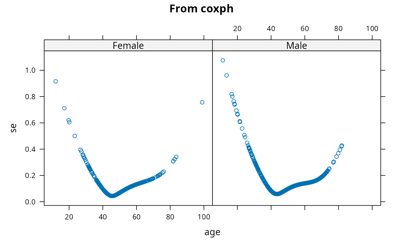
se <- predict(f2, se.fit=TRUE)$se.fit
xyplot(se ~ age | sex, main='From coxph')

comb <- data.frame(age=rep(a, each=2), age2=rep(a, each=2)^2,
                   sex=rep(levels(sex), 3))
p <- predict(f2, newdata=comb, se.fit=TRUE)
comb$yhat <- p$fit
comb$se   <- p$se.fit
comb$lower <- p$fit - z*p$se.fit
comb$upper <- p$fit + z*p$se.fit
comb
#>   age age2    sex    yhat     se   lower  upper
#> 1  30  900 Female -1.0414 0.3084 -1.6458 -0.437
#> 2  30  900   Male -1.0665 0.3111 -1.6762 -0.457
#> 3  50 2500 Female  0.0964 0.0683 -0.0375  0.230
#> 4  50 2500   Male  0.0966 0.0979 -0.0953  0.289
#> 5  70 4900 Female  0.7957 0.1780  0.4469  1.145
#> 6  70 4900   Male  1.0423 0.1880  0.6738  1.411


# g <- cph(Surv(hospital.charges) ~ age, surv=TRUE)
# Cox model very useful for analyzing highly skewed data, censored or not
# m <- Mean(g)
# m(0)                           # Predicted mean charge for reference age


#Fit a time-dependent covariable representing the instantaneous effect
#of an intervening non-fatal event
rm(age)
set.seed(121)
dframe <- data.frame(failure.time=1:10, event=rep(0:1,5),
                     ie.time=c(NA,1.5,2.5,NA,3,4,NA,5,5,5), 
                     age=sample(40:80,10,rep=TRUE))
z <- ie.setup(dframe$failure.time, dframe$event, dframe$ie.time)
S <- z$S
ie.status <- z$ie.status
attach(dframe[z$subs,])    # replicates all variables

f <- cph(S ~ age + ie.status, x=TRUE, y=TRUE)  
#> Error in Design(data, formula, specials = c("strat", "strata")): dataset dd not found for options(datadist=)
#Must use x=TRUE,y=TRUE to get survival curves with time-dep. covariables


#Get estimated survival curve for a 50-year old who has an intervening
#non-fatal event at 5 days
new <- data.frame(S=Surv(c(0,5), c(5,999), c(FALSE,FALSE)), age=rep(50,2),
                  ie.status=c(0,1))
g <- survfit(f, new)
#> Error: object 'f' not found
plot(c(0,g$time), c(1,g$surv[,2]), type='s', 
     xlab='Days', ylab='Survival Prob.')
#> Error: object 'g' not found
# Not certain about what columns represent in g$surv for survival5
# but appears to be for different ie.status
#or:
#g <- survest(f, new)
#plot(g$time, g$surv, type='s', xlab='Days', ylab='Survival Prob.')


#Compare with estimates when there is no intervening event
new2 <- data.frame(S=Surv(c(0,5), c(5, 999), c(FALSE,FALSE)), age=rep(50,2),
                   ie.status=c(0,0))
g2 <- survfit(f, new2)
#> Error: object 'f' not found
lines(c(0,g2$time), c(1,g2$surv[,2]), type='s', lty=2)
#> Error: object 'g2' not found
#or:
#g2 <- survest(f, new2)
#lines(g2$time, g2$surv, type='s', lty=2)
detach("dframe[z$subs, ]")
options(datadist=NULL)