Resampling Model Calibration

Uses bootstrapping or cross-validation to get bias-corrected (overfitting- corrected) estimates of predicted vs. observed values based on subsetting predictions into intervals or better on nonparametric or adaptive parametric smoothers. There are calibration functions for Cox (cph), parametric survival models (psm), binary and ordinal logistic models (lrm, orm) and ordinary least squares (ols). For survival models and orm, "predicted" means predicted survival probability at a single time point, and "observed" refers to the corresponding Kaplan-Meier survival estimate, stratifying on intervals of predicted survival, or, the predicted survival probability as a function of transformed predicted survival probability using the flexible hazard regression approach or for orm and probably better, smoothed overlapping moving Kaplan-Meier estimates (see the val.surv.args argument and val.surv function for details). Nonparametric calibration curves are estimated over a regular sequence of predicted values. The fit must have specified x=TRUE, y=TRUE.

See predab.resample for information about confidence limits. Confidence limits for bootstrap overfitting-corrected calibration curves are not computed for psm fits. This is because of calibrate.psm averages over multiple bootstrap loops. This can probably be changed.

The print and plot methods print the mean absolute error in predictions, the mean squared error, and the 0.9 quantile of the absolute error. Here, error refers to the difference between the predicted values and the corresponding bias-corrected calibrated values.

Below, calibrate.default is for the ols and lrm.

Usage

calibrate(fit, ...)
# Default S3 method
calibrate(fit, predy, 
  method=c("boot","crossvalidation",".632","randomization"),
  B=40, bw=FALSE, rule=c("aic","p"),
  type=c("residual","individual"),
  sls=.05, aics=0, force=NULL, estimates=TRUE, pr=FALSE, kint,
  smoother="lowess", digits=NULL, ...) 
# S3 method for class 'cph'
calibrate(fit, cmethod=c('hare', 'KM'),
  method="boot", u, m=150, pred, cuts, B=40, 
  bw=FALSE, rule="aic", type="residual", sls=0.05, aics=0, force=NULL,
  estimates=TRUE,
  pr=FALSE, what="observed-predicted", tol=1e-12, maxdim=5, ...)
# S3 method for class 'orm'
calibrate(fit, 
                        method="boot", u, m=150, pred, B=40,
                        bw=FALSE, rule="aic",
                        type="residual", sls=.05, aics=0, force=NULL,
                        estimates=TRUE, pr=FALSE, what="observed-predicted",
                        val.surv.args=list(method='smoothkm', eps=30),
                        ...)
# S3 method for class 'psm'
calibrate(fit, cmethod=c('hare', 'KM'),
  method="boot", u, m=150, pred, cuts, B=40,
  bw=FALSE,rule="aic",
  type="residual", sls=.05, aics=0, force=NULL, estimates=TRUE,
  pr=FALSE, what="observed-predicted", tol=1e-12, maxiter=15, 
  rel.tolerance=1e-5, maxdim=5, ...)

# S3 method for class 'calibrate'
print(x, B=Inf, ...)
# S3 method for class 'calibrate.default'
print(x, B=Inf, ...)

# S3 method for class 'calibrate'
plot(x, xlab, ylab, subtitles=TRUE, conf.int=TRUE,
 cex.subtitles=.75, riskdist=TRUE, add=FALSE,
 scat1d.opts=list(nhistSpike=200), par.corrected=NULL, ...)

# S3 method for class 'calibrate.default'
plot(x, xlab, ylab, xlim, ylim,
  legend=TRUE, subtitles=TRUE, cex.subtitles=.75, riskdist=TRUE,
  scat1d.opts=list(nhistSpike=200), ...)

Arguments

fit: a fit from ols, lrm, cph or psm
x: an object created by calibrate
method, B, bw, rule, type, sls, aics, force, estimates: see validate. For print.calibrate, B is an upper limit on the number of resamples for which information is printed about which variables were selected in each model re-fit. Specify zero to suppress printing. Default is to print all re-samples.
cmethod: method for validating survival predictions using right-censored data. The default is cmethod='hare' to use the hare function in the polspline package. Specify cmethod='KM' to use less precision stratified Kaplan-Meier estimates. If the polspline package is not available, the procedure reverts to cmethod='KM'.
u: the time point for which to validate predictions for survival models. For cph fits, you must have specified surv=TRUE, time.inc=u, where u is the constant specifying the time to predict.
m: group predicted u-time units survival into intervals containing m subjects on the average (for survival models only)
pred: vector of predicted survival probabilities at which to evaluate the calibration curve. By default, the low and high prediction values from datadist are used, which for large sample size is the 10th smallest to the 10th largest predicted probability.
cuts: actual cut points for predicted survival probabilities. You may specify only one of m and cuts (for survival models only)
pr: set to TRUE to print intermediate results for each re-sample
what: The default is "observed-predicted", meaning to estimate optimism in this difference. This is preferred as it accounts for skewed distributions of predicted probabilities in outer intervals. You can also specify "observed". This argument applies to survival models only.
tol: criterion for matrix singularity (default is 1e-12)
maxdim: see hare
maxiter: for psm, this is passed to survreg.control (default is 15 iterations)
rel.tolerance: parameter passed to survreg.control for psm (default is 1e-5).
predy: a scalar or vector of predicted values to calibrate (for lrm, ols). Default is 50 equally spaced points between the 5th smallest and the 5th largest predicted values. For lrm the predicted values are probabilities (see kint).
kint: For an ordinal logistic model the default predicted probability that \(Y\geq\) the middle level. Specify kint to specify the intercept to use, e.g., kint=2 means to calibrate \(Prob(Y\geq b)\), where \(b\) is the second level of \(Y\).
val.surv.args: a list containing arguments to send to val.surv when running calibrate.orm. By default smoothed overlapping windows of Kaplan-Meier estimates are used for orm. The val.surv.args argument is especially useful for specifying bandwidths and the movStats eps argument.
smoother: a function in two variables which produces \(x\)- and \(y\)-coordinates by smoothing the input y. The default is to use lowess(x, y, iter=0).
digits: If specified, predicted values are rounded to digits digits before passing to the smoother. Occasionally, large predicted values on the logit scale will lead to predicted probabilities very near 1 that should be treated as 1, and the round function will fix that. Applies to calibrate.default.
...: other arguments to pass to predab.resample, such as conf.int, group, cluster, and subset. Also, other arguments for plot.
xlab: defaults to "Predicted x-units Survival" or to a suitable label for other models
ylab: defaults to "Fraction Surviving x-units" or to a suitable label for other models
xlim,ylim: 2-vectors specifying x- and y-axis limits, if not using defaults
subtitles: set to FALSE to suppress subtitles in plot describing method and for lrm and ols the mean absolute error and original sample size
conf.int: set to FALSE to suppress plotting 0.95 confidence intervals for Kaplan-Meier estimates
cex.subtitles: character size for plotting subtitles
riskdist: set to FALSE to suppress the distribution of predicted risks (survival probabilities) from being plotted
add: set to TRUE to add the calibration plot to an existing plot
scat1d.opts: a list specifying options to send to scat1d if riskdist=TRUE. See scat1d.
par.corrected: a list specifying graphics parameters col, lty, lwd, pch to be used in drawing overfitting-corrected estimates. Default is col="blue", lty=1, lwd=1, pch=4.
legend: set to FALSE to suppress legends (for lrm, ols only) on the calibration plot, or specify a list with elements x and y containing the coordinates of the upper left corner of the legend. By default, a legend will be drawn in the lower right 1/16th of the plot.

Value

matrix specifying mean predicted survival in each interval, the corresponding estimated bias-corrected Kaplan-Meier estimates, number of subjects, and other statistics. For linear and logistic models, the matrix instead has rows corresponding to the prediction points, and the vector of predicted values being validated is returned as an attribute. The returned object has class "calibrate" or "calibrate.default". plot.calibrate.default invisibly returns the vector of estimated prediction errors corresponding to the dataset used to fit the model.

Side Effects

prints, and stores an object pred.obs or .orig.cal

Details

If the fit was created using penalized maximum likelihood estimation, the same penalty and penalty.scale parameters are used during validation.

See https://www.fharrell.com/post/bootcal/ for simulations of the accuracy of various smoothers for binary logistic model calibration, as well as simulations of confidence interval coverage.

Author

Frank Harrell
Department of Biostatistics
Vanderbilt University
fh@fharrell.com

Examples

require(survival)
set.seed(1)
n <- 200
d.time <- rexp(n)
x1 <- runif(n)
x2 <- factor(sample(c('a', 'b', 'c'), n, TRUE))
f <- cph(Surv(d.time) ~ pol(x1,2) * x2, x=TRUE, y=TRUE, surv=TRUE, time.inc=1.5)
#or f <- psm(S ~ \dots)
pa <- requireNamespace('polspline')
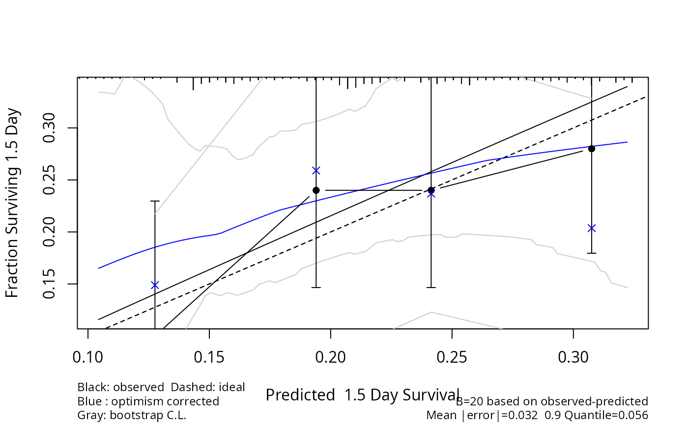
if(pa) {
 cal <- calibrate(f, u=1.5, B=20)  # cmethod='hare'
 plot(cal)
}
#> Using Cox survival estimates at 1.5 Days
cal <- calibrate(f, u=1.5, cmethod='KM', m=50, B=20)  # usually B=200 or 300
#> Using Cox survival estimates at 1.5 Days
plot(cal, add=pa)


set.seed(1)
y <- sample(0:2, n, TRUE)
x1 <- runif(n)
x2 <- runif(n)
x3 <- runif(n)
x4 <- runif(n)
f <- lrm(y ~ x1 + x2 + x3 * x4, x=TRUE, y=TRUE)
cal <- calibrate(f, kint=2, predy=seq(.2, .8, length=60), 
                 group=y)
# group= does k-sample validation: make resamples have same 
# numbers of subjects in each level of y as original sample

plot(cal)

#> 
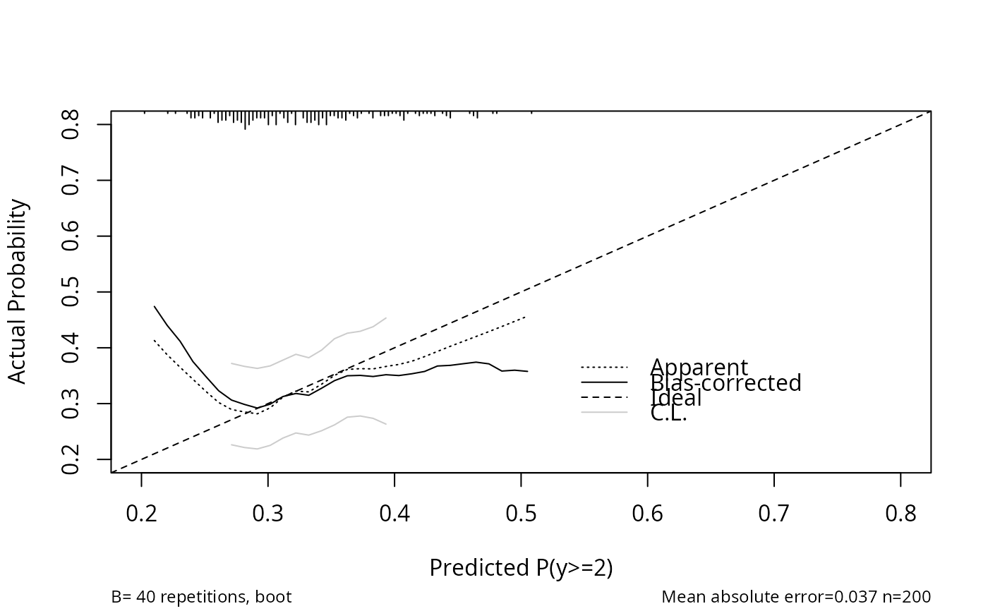#> n=200   Mean absolute error=0.037   Mean squared error=0.003
#> 0.9 Quantile of absolute error=0.09
#> 
#See the example for the validate function for a method of validating
#continuation ratio ordinal logistic models.  You can do the same
#thing for calibrate